TL;DR: This is a release post for ThunderKittens 2.0, our cute little CUDA-embedded DSL, along with a technical deep dive for those who are interested.
Since releasing ThunderKittens (TK) two years ago, we've spent most of our time adding new features: for instance, boilerplate templates, custom on-device schedulers, Blackwell support, FP8 support, multi-GPU support, and Megakernels.
This release is different in that it's as much about subtraction as addition: we refactored the internals, hunted down unnecessary memory instructions and assembler inefficiencies, reduced build system complexities, and identified many surprising behaviors on modern Nvidia GPUs that guide how kernels should not be optimized.
Thus, the goal of this post is to briefly announce the release, and then share some of our learnings. On the release side, ThunderKittens 2.0 brings:
- New features: MXFP8/NVFP4 support, CLC scheduling, tensor memory controllability, many new utilities, PDL, and more.
- Major refactor of the internal code, during which we found a number of subtle inefficiencies described throughout the rest of this post.
- Much simpler build structure for all of our example kernels, so you (or your agent) can easily adapt them for your own use!
- Contributions from industry: many companies have their own internal fork of ThunderKittens, and many were generous enough to contribute them back to us!
These changes enabled us to write even faster kernels with new optimization strategies and fewer lines of code. As an example, we present the new state-of-the-art BF16 / MXFP8 / NVFP4 GEMM kernels that surpass or match cuBLAS performance on Nvidia B200s:
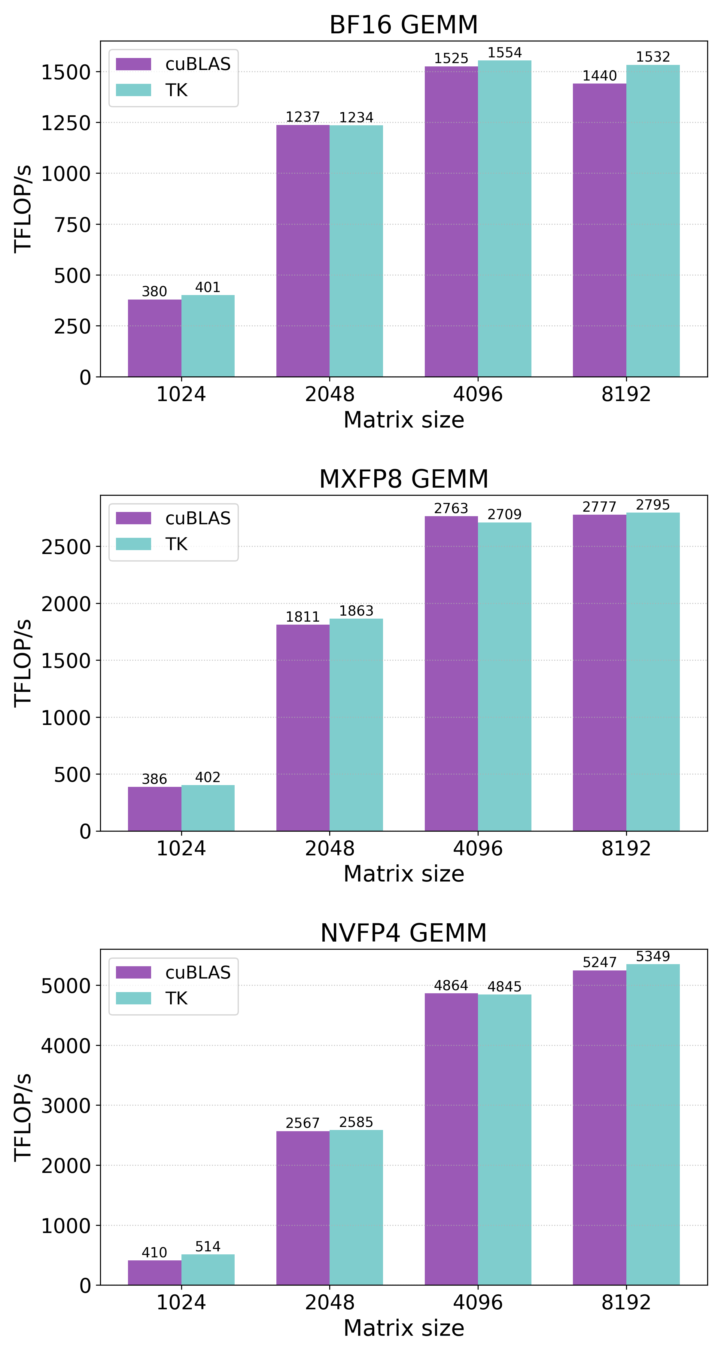
Figure 1: New Kernels! All of the kernels (both TK and cuBLAS) were benchmarked using bitwise-identical random inputs with 500 warmup iterations, 100 profiling iterations, and L2 cache eviction. Details on the benchmarking method are described later in this post.
We also updated all of our existing example kernels to use the newer APIs, and are actively implementing more state-of-the-art kernels with TK (e.g., Flash Attention 4, grouped GEMMs, GEMV).
That's it for the release! Please check out our repository for the details. The rest of this post cherry-picks some of the interesting technical details we found while optimizing TK. Specifically, we'll discuss:
- Memory consistency. Can't escape it if you want to squeeze out the last few TFLOPs! Tightening memory synchronization with proper reasoning is crucial to getting peak performance.
- Tensor core and memory pipelining. Some tensor core instructions are implicitly pipelined without proper documentation, and the best memory pipelining strategy for the given workload might not be so obvious.
- Hinting the PTX assembler properly. It really doesn't trust us otherwise! Logically identical code can produce meaningfully different instructions depending on how it's written.
- Occupancy. Don't trust what the code suggests; distributed shared memory does not work identically across all SMs, and tensor core instructions silently limit occupancy.
- Benchmarking GPU kernels correctly, with L2 usage and power consumption in mind.
We deliberately chose topics that are interesting and not well-covered elsewhere. These are the last bits to really squeeze out everything. For obtaining the first 90% of TFLOPs, we recommend reading this great blog post from Modular.
Memory consistency
CUDA/PTX provides many different kinds of memory consistency primitives. Missing memory synchronization leads to race conditions, while unnecessary ones lead to a loss of TFLOPs. In fact, tightening the acquire/release pattern usage was one of the last optimizations required for our Megakernel implementation to surpass SGLang: we observed that a few loose fence instructions caused over 10% loss in performance.
Here, we'll demonstrate how we reason about using the memory fence and how it can lead to performance improvements. As a running example for this section, ThunderKittens previously included the following code in its Blackwell blockscaled tensor core matrix multiplication path (the mma(...) function):
... // Prepare instruction and matrix descriptors

asm volatile("tcgen05.fence::after_thread_sync;\n");
asm volatile("fence.proxy.async.shared::cta;\n" ::: "memory");

... // Perform tcgen05.mma
To provide a brief background on what is happening here: this code is performing the 5th generation tensor core matrix multiplication. The operands A and B matrix tiles reside in shared memory, and the output is accumulated onto tensor memory. In addition, this performs blockscaled matrix multiplies (e.g., MXFP8 or NVFP4); thus, the input scales for A and B reside in the tensor memory as well. Fully understanding blockscaled matrix multiplication does not really matter here, but you can read more about it in this other blog post if you are interested.
So why the two fence instructions? Before the tensor cores begin consuming data (upon issuance of tcgen05.mma), we need to ensure that all inputs are loaded to their respective locations (tensor memory and shared memory) and are visible to the tensor cores. These fences serve as safety measures guaranteeing that all preceding loads and copies have completed and their effects are visible.
However, profiling this path revealed that the two fences cost roughly 20-30 TFLOPs in compute throughput of the GEMM kernel. So the natural question was: do we actually need them?
Understanding the PTX memory consistency model
To understand what these fences do in the first place, we must understand the PTX memory consistency model better.
In PTX, a memory write to shared or global memory by one thread is guaranteed to be visible to reads by other threads, provided the write and read are ordered by causality. Two memory operations X and Y are causally ordered if:
- X and Y are issued by the same thread,
- X synchronizes with Y, or
- There is another operation Z between X and Y, where X-Z and Z-Y are ordered by causality (transitivity).
We say “X synchronizes with Y” if either (1) X and Y are both barrier operations (bar/barrier) executed on the same barrier, or (2) if X is write-release, Y is read-acquire, and Y observes the value written by X. There are additional nuances and cases on this, but these should suffice for the purposes of this post.
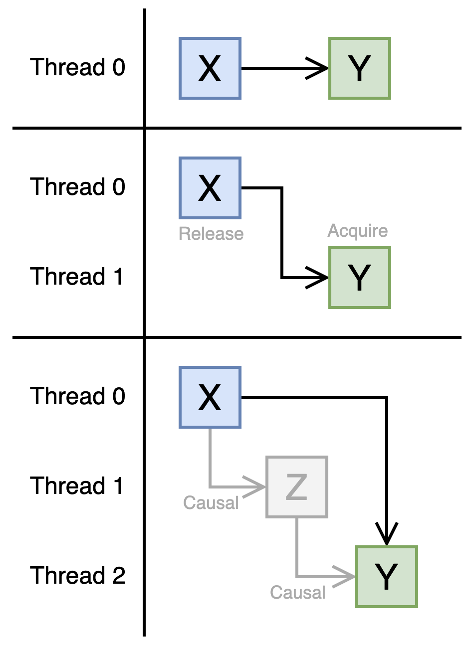
Figure 2: Examples of memory operations ordered by causality in PTX.
There is also an additional concept of memory proxy. A proxy refers to a group of memory access methods. Most memory operations (e.g., st, ld) use the generic proxy. However, some asynchronous operations like tcgen05.mma or cp.async.bulk.tensor (TMA) use the async proxy. The above causality ordering only holds within the same proxy. In order for causality to hold between two different proxies, a proxy fence (fence.proxy) instruction must be inserted in between.
Can the tensor cores observe the inputs?
By the time the tensor cores begin matrix multiplication (via the issuance of the tcgen05.mma instruction), they must be able to observe:
- The input A and B tiles, loaded through TMA into shared memory (i.e., through the
cp.async.bulk.tensorinstruction). - The input scales, loaded through the
tcgen05.cpinstruction into tensor memory.
Note that the tensor cores must also observe that the epilogue threads are no longer accessing the accumulator, but we set that aside for this post.
We must fully understand what happens between the writes (cp.async.bulk.tensor and tcgen05.cp) and the read (tcgen05.mma), and to determine whether the inputs are guaranteed to be visible to the tensor cores. Answering this requires collecting and combining information scattered across several parts of the PTX documentation, then reasoning about it carefully. Below, we cite the relevant sections as we go.
First, can the tensor cores observe the shared memory filled by TMA? Let's work through this step by step.
- The first thing that happens is memory copy operation from global memory to shared memory. This happens as part of the TMA load instruction (
cp.async.bulk.tensor) and is a weak memory operation (section 9.7.9.27.1.2) performed through the async proxy (section 9.7.9.25.2). - As part of the same TMA load instruction, an
mbarriercomplete-txoperation follows immediately. This operation is implicitly ordered with regard to the preceding memory copy operation (section 8.9.1.1) and is a release operation (section 9.7.9.27.1.2). Also, an implicit generic-async proxy fence is inserted right after completion (section 9.7.9.25.2). - The
mbarriertry-waitoperation that precedes the tensor core matrix multiplication is, by default, an acquire operation (section 9.7.13.15.16), and ThunderKittens uses exactly this default behavior. Thus, this establishes a causality order with the TMA load. - Finally, the
tcgen05.mmainstruction executes in the same thread that issued thembarrer try-waitinstruction, preserving the causality order, and reads from shared memory through the async proxy (section 9.7.16.6.5), the same proxy used bycp.async.bulk.tensor.
The verdict is that, for this specific scenario, causality order is already established between the TMA write and the tensor core read due to transitivity! No additional memory fences are needed for the shared memory read. One down, one to go.
Second, can the tensor cores observe the tensor memory filled in by tcgen05.cp?
- According to section 9.7.16.6.2,
tcgen05.mmais implicitly pipelined with regard totcgen05.cp(we discuss this in more detail in the next section). - According to section 9.7.16.6.4.1, implicitly pipelined instructions do not require a memory ordering mechanism.
Combining these two facts, we can conclude that tcgen05.cp and tcgen05.mma, when issued by the same thread, are automatically well-ordered with respect to each other. As we will explain shortly, this is a canonical pattern for writing blockscaled GEMM kernels (and we have not found a case where issuing these instructions from different threads is beneficial). The fence that would otherwise ensure visibility of tcgen05.cp to tcgen05.mma (i.e., after_thread_sync in the example code above) is therefore unnecessary.
This is great. Neither of the two memory fences were needed. Removing unnecessary fences like these here and there gave us roughly a 20 TFLOP/s boost across our GEMM and attention kernels.
Tensor core/memory pipelining
Pipelining tcgen05.cp with tcgen05.mma
For our MXFP8/NVFP4 kernels, the major bottleneck was loading scale values into tensor memory.
Apologies in advance for throwing a bunch of numbers at you, but this is needed for the discussion: MXFP8 uses one scale value per 32 elements, and NVFP4 uses one per 16 elements. To fully utilize the tensor cores, Blackwell GPUs require a 128x128x32 GEMM shape per CTA for MXFP8 and 128x128x64 for NVFP4. The canonical way to pipeline tcgen05.mma is to provide enough data for 4 consecutive MMAs without interruption; that is, 128x128x128 per CTA for MXFP8 and 128x128x256 for NVFP4. We call these 4 consecutive MMAs one MMA stage.
From these numbers, we can derive the following (we disregard scale swizzling for this post):
- We need
128 * 128 / 32 = 512scale values per operand per MMA stage per CTA for MXFP8. - We need
128 * 256 / 16 = 2048scale values per operand per MMA stage per CTA for NVFP4.
The problem is that blockscaled MMA needs the same scale values to be broadcasted to all 4 warps in tensor memory, and only one instruction supports this: tcgen05.cp.32x128.warpx4. As its name suggests, this copies only 32 * 128 / 8 = 512 values per invocation (the 128 refers to bytes). This is great for MXFP8: a single tcgen05.cp per operand is enough to feed one tensor core MMA stage.
For NVFP4, however, this means you need 4 tcgen05.cp instructions per MMA stage just to supply one operand. With both A and B, that doubles. Then, due to a subtle layout detail on the B side, the B matrix requires an additional 2x factor, bringing the total to 12 tcgen05.cp instructions per MMA stage.
That's a lot, and our original kernel design looked something like this:
if (warp_id == 0) {
    Load A and B tiles with TMA (HBM -> SMEM)
} else if (warp_id == 1) {
    Load A and B scales with TMA (HBM -> SMEM)
} else if (warp_id == 2) {
    Wait for A and B scales to arrive at SMEM
    Load A and B scales with tcgen05.cp (SMEM -> TMEM)
} else if (warp_id == 3) {
    Wait for A and B tiles to arrive at SMEM
    Wait for A and B scales to arrive at TMEM
    Run 4 MMAs
}
In the pseudocode above, warp_id == 2 would need to issue 12 tcgen05.cp instructions per MMA stage, and warp_id == 3 would then have to explicitly wait for all of them to complete. With these overheads, our kernel throughput suffered badly, roughly 10% lower than that of state-of-the-art kernels.
However, after a few weeks of struggling, something caught our eyes:
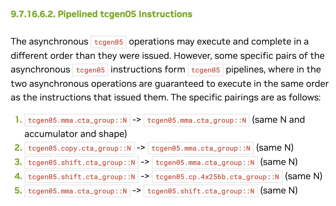
Figure 3: PTX documentation section 9.7.16.2.
Notice how it describes that the tcgen05.copy instruction is implicitly pipelined with respect to tcgen05.mma. We had read the PTX documentation countless times, but only at this point did we realize that tcgen05.copy was a typo of tcgen05.cp; the hypothetical tcgen05.copy instruction never appears again anywhere in the document. The lack of any example showing tcgen05.cp pipelined with tcgen05.mma compounded the confusion, preventing us from realizing this for a surprisingly long time.
With this new knowledge, we arrived at a new design. By merging the copy and MMA work into the same thread and removing the now-unnecessary barrier waits, we recovered the missing ~500 TFLOP/s, roughly a 10% improvement for NVFP4 GEMM.
if (warp_id == 0) {
  Load A and B tiles with TMA (HBM -> SMEM)
} else if (warp_id == 1) {
  Load A and B scales with TMA (HBM -> SMEM)
} else if (warp_id == 3) {
  Wait for A and B tiles to arrive at SMEM
  Wait for A and B scales to arrive at SMEM
  Load A and B scales with tcgen05.cp (SMEM -> TMEM)
  Run 4 MMAs
}
Pipelining tensor memory
A common pattern described in many writings is to pipeline MMA with tensor memory reads. The key idea is this: tensor memory is organized as a 128x512 array, and non-blockscaled tcgen05.mma instructions accumulate into at most 128x256 of the tensor memory at a time. So, the natural approach is to alternate between the two 128x256 slots, such that one is used by the tensor cores for accumulation, and the other is used by epilogue threads to read out the results of the previous MMA operation.
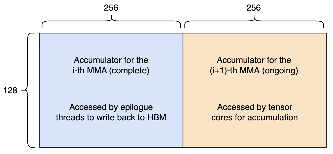
Figure 4: Tensor memory buffering. The 128x512 tensor memory per SM is divided into two slots: one accessed by tensor cores, the other accessed by epilogue threads simultaneously.
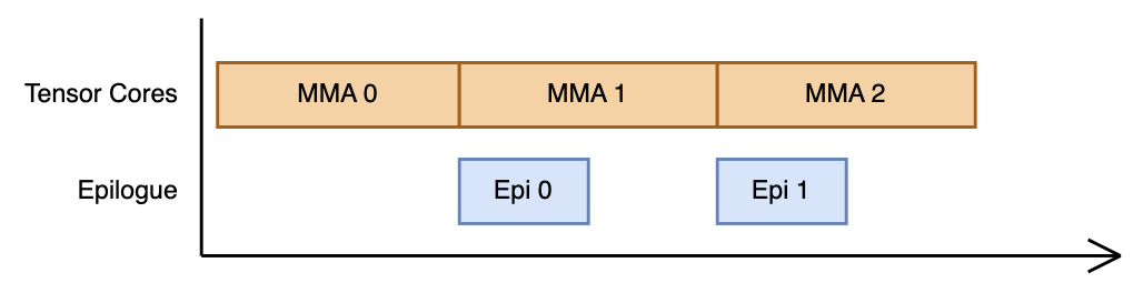
Figure 5: Visualization of the resulting pipeline from the above buffering scheme.
This is theoretically sound in that there exists no “pipeline bubble” where the tensor cores sit idle waiting for the epilogue threads to finish. In practice, we found this to be the most efficient choice for small GEMM sizes (roughly below 2048x2048x2048).
For larger sizes, however, we found "double accumulation" pattern to work better. In this scheme, we run two MMA pipelines simultaneously, both sharing the same A tile while operating on different B tiles. This means we accumulate across the entire 128x512 tensor memory throughout, and the tensor cores wait while the epilogue threads drain it.
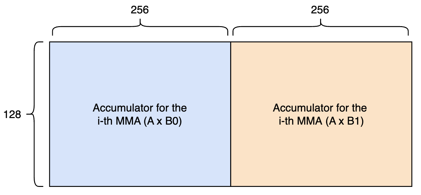
Figure 6: An alternative tensor memory buffering scheme. The 128x512 tensor memory per SM is divided into two slots, both accessed by either the tensor cores or the epilogue threads.
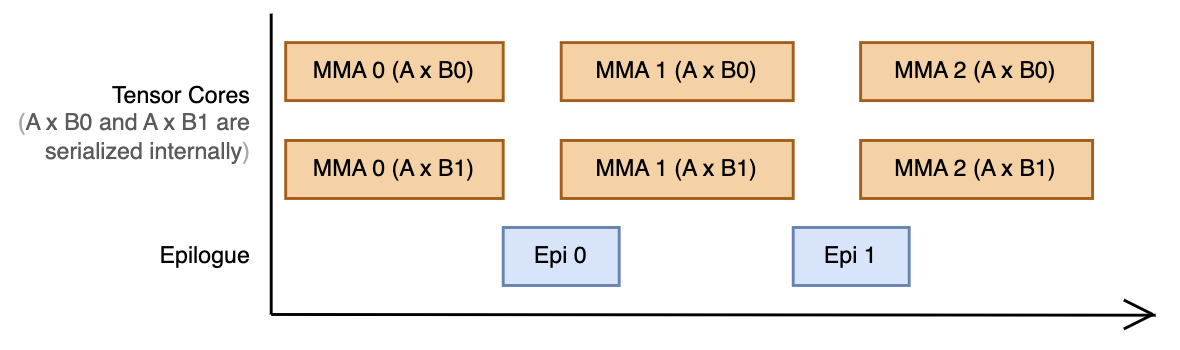
Figure 7: Visualization of the resulting pipeline. Note that A x B0 and A x B1 are serialized internally at the tensor core hardware, but this is omitted from the diagram for simplicity.
This introduces a slight bubble between MMAs: the tensor cores must wait for the epilogue threads to read all 256 KB (128 * 512 * 4 bytes per element) from tensor memory before starting the next operation. But the reduced memory traffic from sharing the A tile compensates for larger GEMMs, giving us an additional ~100 TFLOP/s for our BF16 GEMM kernel.
PTX assembler behavior on SM90+ single-threaded instructions
Special thanks to Nash Brown for identifying this!
A common pattern in modern GPU kernels is to perform warp specialization where each warp is assigned a single role. On Hopper and Blackwell GPUs, many of these roles only require a single thread issuing instructions within the warp. For instance, a "loader" warp issues TMA loads, which need only one thread. The usual ThunderKittens pattern looks like this:
if (warpgroup::groupid() == 0) {
    if (warpgroup::warpid() == 0 && warp::laneid() == 0) {
        tma::expect_bytes(arrived, sizeof(smem));
        tma::load_async(smem, A, {0, 0}, arrived);
    }
}
Here, arrived is an mbarrier object and smem is a shared memory tile. To those unfamiliar with ThunderKittens, this code selects the first warpgroup's first warp, then lane 0 within that warp. This makes sense at the source level since TMA only needs to be issued by a single thread.
But when you inspect the SASS generated by this code, it looks like the following:
0x0260 @P0 ELECT P1, URZ, PT ;
0x0270     UTMALDG.5D [UR8], [UR4] ;
0x0280 @P1 PLOP3.LUT P0, PT, P1, PT, PT, 0x8, 0x80 ;
0x0290     PLOP3.LUT P1, PT, PT, PT, PT, 0x8, 0x80 ;
0x02a0 @P0 BRA.U.ANY 0x260 ;
Note that this code is already guarded by warpgroup::warpid() == 0 && warp::laneid() == 0, so only a single thread can reach it. Yet the PTX assembler has inserted a loop: it elects a thread, issues the TMA load, removes that thread from the active set, branches back to 0x0260, elects another from the remaining 31, and repeats, cycling through all 32 threads in turn. In practice, however, only one thread ever executes this section of code.
Why does this happen? There are two reasons: (1) the UTMALDG instruction (SASS equivalent for TMA load) cannot be issued by multiple threads of the same warp simultaneously, and (2) the PTX assembler cannot prove that this code path is reached by only a single thread, so it conservatively inserts a serialization loop.
How can we avoid this? We must use an instruction that the PTX assembler knows selects exactly one thread: the elect.sync instruction. This PTX instruction elects a single thread from the current warp. The effect is the same as warp::laneid() == 0, but the assembler recognizes the intent and avoids the loop.
In ThunderKittens, you can use the warp::elect_leader() function to do this. If you change the code like the following:
if (warpgroup::groupid() == 0) {
    if (warpgroup::warpid() == 0 && warp::elect_leader()) {
        tma::expect_bytes(arrived, sizeof(smem));
        tma::load_async(smem, A, {0, 0}, arrived);
    }
}
The generated SASS changes to:
0x01e0*/      ELECT P0, URZ, PT ;
0x01f0*/ @!P0 BRA 0x2d0 ;
... (address calculation)
0x02b0*/      UTMALDG.5D [UR8], [UR4] ;
0x02d0*/      BSYNC.RECONVERGENT B0 ;
No loops! By applying this pattern to all single-threaded instructions across our kernels, we were able to improve compute throughput by up to 10% for small-shaped GEMMs.
Occupancy
Here we describe a few of our failure modes, so you don't fall into the same traps :\
Not all SMs support all cluster sizes
Threadblock clusters larger than 2 can improve compute throughput by enabling distributed shared memory and reducing memory controller traffic. But there was a caveat: some cluster sizes prevent the scheduler from fully utilizing all SMs.
What does this even mean? Suppose we want to implement a persistent grid kernel on a B200 GPU. The B200 has 148 SMs, so a natural pattern is to set the grid size to 148, have each threadblock consume most or all of an SM's shared memory, specify the cluster size via __cluster_dims__(n), and launch.
Now, this works well if you have a cluster size of 2: each SM pair forms a cluster, and you have a total of 148 / 2 = 74 threadblock clusters running.
But what about a cluster size of 4? We would expect groups of 4 SMs to team up, giving 148 / 4 = 37 clusters, right?
To test this, we can have a kernel print its cluster and block information, sleep for a noticeable duration, and return:
__global__ __cluster_dims__(2) void kernel(const __grid_constant__ globals<C> g) {
    printf("num_clusters=%d, cluster_idx=%d, cluster_size=%d, cta_rank=%d, blockIdx.x=%d\n", nclusterid().x, clusterIdx().x, cluster_nctarank(), cluster_ctarank(), blockIdx.x);
    for (int i = 0; i < 500000; i++) __nanosleep(10000);
}
If you run this code, you'll see that the result is quite surprising: only 132 SMs are active at a time. The remaining 16 threadblocks are scheduled only after the first 132 exit. This was quite strange, so we decided to see how it behaves for all powers-of-2 cluster sizes:
| Cluster Size | Active SMs |
|---|---|
| 2 (grid size 148) | 148 |
| 4 (grid size 148) | 132 |
| 8 (grid size 144) | 120 |
| 16 (grid size 144) | 112 |
Table 1. Active SMs by cluster size on B200.
This implies that blindly setting a cluster size greater than 2 on a persistent grid kernel produces a mysterious slowdown that can take some time to diagnose. Our hypothesis is that distributed shared memory requires internal wiring between the SMs and it was a hardware engineering decision to choose not to wire certain SMs for simpler implementation.
Does this mean Nvidia fooled us with threadblock clusters and distributed shared memory? The __cluster_dims__() attribute is certainly misleading, but no. It turns out that by not using __cluster_dims__ and instead launching kernels with cudaLaunchKernelEx, you gain the ability to specify two cluster sizes: a preferred size and a minimum size.
The scheduler first fills SMs using the preferred cluster size (e.g., 132 SMs filled with 4-clusters), then uses the minimum cluster size to fill the remainder. The kernel must be written to support both sizes. In ThunderKittens 2.0, we added the LaunchConfig utility for this purpose (it is a thin wrapper around the CUDA API, so feel free to use the API directly if you prefer).
TCGEN05 instructions hard-limit per-SM occupancy
Another surprising thing we found was that the moment a kernel accesses tensor memory, its maximum per-SM occupancy is hard-limited to 1. We can see this with a simple test code:
__global__ void empty_kernel() {}
__global__ void tcgen05_kernel() {
    __shared__ uint32_t tmem_addr;
    asm volatile(
        "{tcgen05.alloc.cta_group::1.sync.aligned.shared::cta.b32  [%0], %1;}"
    ::  "l"(reinterpret_cast<uint64_t>(&tmem_addr)), "n"(128)
    );
}

void print_occupancy(const char* name, const void* kernel, int block_size) {
    int max_blocks_per_sm = -1;
    CUDACHECK(cudaOccupancyMaxActiveBlocksPerMultiprocessor(
        &max_blocks_per_sm,
        kernel,
        block_size,
        0
    ));
    printf("%s: Max blocks per SM: %d\n", name, max_blocks_per_sm);
}

int main() {
    const int block_size = 256;
    print_occupancy("empty_kernel", reinterpret_cast<const void*>(empty_kernel), block_size);
    print_occupancy("tcgen05_kernel", reinterpret_cast<const void*>(tcgen05_kernel), block_size);
    return 0;
}
When you compile and run the above code, the output shows that tcgen05_kernel has a maximum occupancy of 1 block per SM. This is quite surprising since the kernel allocates only one quarter of the available tensor memory, and all tensor memory allocation and management instructions in PTX implicitly suggest that tensor memory is designed to be shared among multiple resident blocks. Nonetheless, it appears that increasing per-SM occupancy is not a viable optimization strategy when utilizing tensor cores in a Blackwell kernel.
Benchmarking GPU kernels properly
After weeks of benchmarking GEMM kernels, one thing that consistently bothered us was the seemingly unbeatable speed of CUTLASS GEMM kernels when benchmarked with their own profiler (the CUTLASS Profiler). They were consistently 100-150 TFLOPs faster than ours. At one point, we were adding the prefix "cutlass" to our kernel names and were half-convinced that Nvidia had private assembler optimization passes reserved for their own code.
Fortunately, there was no such thing for this case. But it did turn out that the CUTLASS Profiler, by default, rounds input values to nearest integers before passing them to the kernels. Aside from the fact that this is a questionable design choice, this heavily affects the performance. Integer-like input matrices produce less bit-flipping in the GPU's transistors, which reduces power consumption and, consequently, the likelihood of clock throttling.
This triggered us to investigate further, we realized just how many factors can influence observed TFLOPs. Every subtle benchmark design decision matters: using 2 CUDA events versus N*2 (where N is the number of profiling iterations), how you clear L2 cache between iterations (explicit flush vs natural eviction through input groups), benchmarking from C++ versus PyTorch, what random distribution and seed you use, and so on.
In our experience, the set of design choices described above can account for up to a 10% difference in results. After a series of experiments, we settled on the following convention for benchmarking our kernels and reporting performance numbers publicly:
- Use bitwise identical random inputs (usually from uniform distribution; range depends on the precision being used).
- If the total input size is less than 3x the L2 cache size (e.g., 128 MB on B200), use multiple input groups. This way, each group's data naturally evicts the previous group's residency in L2, simulating cold-cache conditions. We found that explicit cache flushing meaningfully slows down the measured time even with proper CUDA event usage.
- Run 500 warmup iterations before profiling, to reach a power-steady state.
- Run 100 profiling iterations, with the kernels launched back-to-back without intermediate synchronization.
- Measure time using 2 CUDA events recorded immediately before and after all of the profiling iterations.
- Give GPUs short idle period between benchmarking two kernels, to allow thermal cooldown.
We encourage adopting and/or improving this convention. The pseudocode below illustrates the approach. Note that even though this code is in CUDA C++, it's also fully possible to do exactly the same in PyTorch through the torch.cuda API:
int l2_cache_size;
cudaDeviceGetAttribute(&l2_cache_size, cudaDevAttrL2CacheSize, 0);
int num_input_groups = (input_size >= l2_cache_size * 3) ? 1 : int(l2_cache_size * 3 / input_size) + 1;

// <Prepare `num_input_groups` set of inputs, ensuring they are bitwise-identical for all kernels being benchmarked>

cudaDeviceSynchronize();

for (int i = 0; i < 500; i++) {
    input_group_index = i % num_input_groups;
    launch_kernel(inputs[input_group_index]);
}

cudaEventRecord(start_event);

for (int i = 0; i < 100; i++) {
    input_group_index = i % num_input_groups;
    launch_kernel(inputs[input_group_index]);
}

cudaEventRecord(end_event);
cudaEventSynchronize(end_event);

float milliseconds;
cudaEventElapsedTime(&milliseconds, start_event, end_event);

// <Save time and throughput>

sleep_ms(500);
What's next?
We're happy to say that ThunderKittens is now fully optimized for Blackwell and can still produce state-of-the-art kernels with significantly fewer lines of code than other CUDA DSLs. We're also happy to see TK 2.0 already being adopted by the industry! For instance, it powers training kernels for Cursor's Composer and inference kernels for Together AI.
Yet there is a variety of wild optimizations that could push these kernels even further. Most importantly, modern GPUs are composed of multiple chiplets, each with its own partition of L2 cache and HBM. The Nvidia B200, for instance, is two chiplets stitched together by a 10 TB/s chip-to-chip interconnect, significantly lower throughput than the L2 itself (roughly 21 TB/s by our measurement). This creates an unavoidable NUMA effect: memory throughput is limited by the interconnect bandwidth even on an L2 hit. If we can get this right, whether through kernel design or model architecture, there's a good chunk of speedup on the table.
And we're not done with Megakernels yet! We've shown that Megakernels deliver significant speedups over state-of-the-art inference engines, even in compute-bound, GPU-friendly workloads like prefill. The remaining question is how to make them accessible. Rather than another DSL or standalone compiler, we believe what's needed is a fundamental change in ML infrastructure. PyTorch is a great frontend for representing compute graphs, and we're extremely grateful for its existence; but its 10+-year-old backend architecture may not be the best fit for extracting every last TFLOP from modern GPUs. We'll see!
As always, if you'd like to learn more or contribute, feel free to reach out to Stuart at ssul@cs.stanford.edu :)
Acknowledgements
We are grateful to Cursor for generously providing the GPUs for this work. We also thank Simran Arora, Simon Guo, and Alex Waitz for their thoughtful feedback on this post.