Dec 11, 2023 · 12 min read
Long Convolutions for GPT-like Models: Polynomials, Fast Fourier Transforms and Causality
We’ve been writing a series of papers (1, 2, 3) that have at their core so-called long convolutions, with an aim towards enabling longer-context models. These are different from the 3x3 convolutions people grew up with in vision because well, they are longer–in some cases, with filters as long as the whole sequence. A frequent line of questions we get is about what these long convolutions are and how we compute them efficiently, so we put together a short tutorial. At the end of this, you’ll remember convolutions, Fast Fourier Transforms (FFTs), and understand how “causality” in this transformation is important to enable GPT-like models.
Convolutions as Polynomial Multiplication
Today, we’re going to consider here a sequence of real numbers . This is like the input to a transformer, a sequence of token embeddings or image patch embeddings, etc. For simplicity, let’s consider . Now, you’ve probably seen pictures like this one that talk about short convolutions, say with a convolution which is an edge detector:
A simple edge detector convolution.
Recall the typical way a convolution is defined between two discrete sequences and :
Let’s do something that seems a little weird at first but will make sense in a bit. We’ll write the sequence as the coefficients of a polynomial , and we’ll write our convolution filter as the coefficients of a polynomial .
Here all we’ve done is notational, we’ve regarded both of the sequences as coefficients in a polynomial. This may seem like fancy notation, but stick with it! Now, let’s multiply these polynomials:
Convince yourself of this equation. Here we have used the convention that the coefficients not explicitly mentioned are zero. That inner term is the convolution from above! That is, the coefficients of are exactly the convolution between the vectors and . So the message is that:
convolution can be defined with polynomial multiplication
In this way, we can extend convolutions of small sequences to arbitrary-sized sequences of convolutions. Here’s an example of a long convolution, where the input filter is as long as the sequence. Here, the convolution filter is built from a simple S4 filter.
A long convolution.
Now, observe that if we multiply a polynomial of degree and together we can get a polynomial of degree . We’ll put a pin in it for now – and circle back at the end when we start talking about different types of convolutions.
Polynomials can be Evaluated
The beautiful thing about polynomials is that they are both a nice discrete object we can understand, but also a function that we can evaluate. This observation is the key to the fast fourier transform. Here’s the crux of the observation:
- We can define a degree n+1$ coefficients as we did above. This is the coefficient representation.
- We can also define a degree polynomial by its values at any points. This is the value representation.
Suppose we took our function f above and evaluated at some points we picked . Let’s convince ourselves there is a simple map. This matrix is called a Vandermonde:
This famous matrix has determinant which is non-zero whenever all the points are distinct. If you’re a linear algebra nerd, you can see that the condition number may be a bit high if we’re not careful about how we pick points–more on that later.
Why is the value representation useful for us? Well imagine we had two value representations of the polynomials and at the same points. Then, note that:
This is a much simpler multiplication: it’s pointwise. Now to exactly reconstruct , we need to evaluate and at points (more later).
Multiplying polynomials can be much faster if they are in the value representation.
So how do we use this? Well this is where the Fast Fourier Transform comes in!
Converting from Coefficients to Values and Back with the FFT
Note that we get to pick the evaluation points. What do we want from those points? Well ideally, we’d like that the transformation is maximally stable. The best we can hope for is that all the eigenvalues have norm as close to 1 as possible. This is where our friend the roots of unity come in:
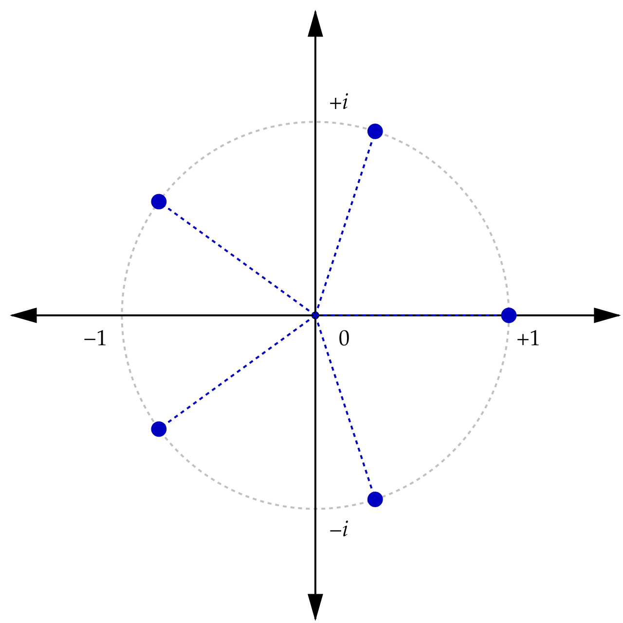
Visualization of roots of unity for n = 5, courtesy Wikipedia.
These characters are great! So we form the Vandermonde with them, and notice that has a very special name–it’s the discrete fourier transform (DFT) matrix. More on that later, but observe that it’s now possible to go back and forth with condition number that is effectively 1.
Now the magic: The DFT can be implemented not by this matrix but by a series of great algorithms, perhaps most famously the Cooley-Tukey algorithm that computes in time using a classic divide-and-conquer algorithm. This is the fast fourier transform (FFT). This gives us a really simple algorithm:
- Take the FFT of the sequence and the filter.
- Point wise multiply.
- Take the inverse FFT.
This is an algorithm. Pretty great! We worked hard to fuse this algorithm and make it efficient on modern hardware – check out FlashFFTConv for a primer there.
Causality in Transforms
One particular issue where this is important is causality. Basically the idea is that the value of a sequence element should depend only on elements that come earlier in the sequence (and not on later ones, as is common in so-called bidirectional models). These causal transformations have become really popular because of GPT’s left-to-right prediction models:
Left-to-right next token prediction with language models.
Now, observe that multiplying polynomials gets this for free! If we multiply a polynomial by convolution then notice that degree k only depends on degrees of the input that are smaller than it (and the filter, which isn’t strictly speaking necessary)!
There’s a catch. Recall from earlier that if we multiply a polynomial of degree d and m together we can get a polynomial of degree d+m. This means we have more coefficients than you might expect. This becomes important when we start using the FFT to do convolutions.
It turns out that there are a few things we can do with those extra terms, and they correspond to different convolution operations we can compute:
- Make the sequence longer. We don’t typically do this in machine learning models because we want to keep the sequence length the same per layer, but we could do this.
- Throw them away. This is equivalent to operating "mod ", if you’re a math nerd. But this is often done.
- Wrap those coefficients around. Here we set and so gets added to . These are sometimes called circular convolutions.
Three options for what to do when multiplying polynomials, and what it means for the resulting convolution.
Thus, to make fourier models GPT-like, we need to adopt the “make it longer” or “chop it off” version of convolutions above (we choose the latter)--not the circular convolution. However, for BERT-style models we might be able to use the wrap-around model. For example, M2-BERT and DiffuSSM use the wrap-around properties to compute a bidirectional convolution, by using a kernel that’s twice as long as the input.1
What's Next
This is really just a first primer into convolutions and their connections to polynomials. The nice thing is – once we’ve made this connection, we can bring the tools of polynomial theory to bear on understanding these ML layers:
- In Monarch Mixer, we used this connection to figure out how to make Monarchs causal.
- In some work to release this week, Simran and Sabri take this polynomial view to the extreme, and show how polynomial circuits can reason about what is computable with convolutions.
This blog is a series of surveys and tutorials on building blocks for AI Systems, associated with an upcoming NeurIPS keynote. If you like this style of work and want to learn more, check out the community we’re building over on this GitHub, and come on in!
Dan Fu: danfu@cs.stanford.edu
- The pure circular version could lead to potentially even faster convolutions based on the discrete cosine transform which is 4x faster since it’s real and it wraps around naturally.↩