One goal of deep learning research is to find the simplest architectures that lead to the amazing results that we've seen for the last few years. In that spirit, we discuss the recent S4 architecture, which we think is simple—the structured state space model at its heart has been the most basic building block for generations of electrical engineers. However, S4 has seemed mysterious—and there are some subtleties to getting it to work in deep learning settings efficiently. We do our best to explain why it's simple, based on classical ideas, and give a few key twists. You can find the code for this blog on GitHub!

Further Reading If you like this blog post, there's a lot of great resources out there explaining and building on S4. Go check some of them out!

• The Annotated S4: A great post by Sasha Rush and Sidd Karamcheti explaining the original S4 formulation.
• S4 Paper: The S4 paper!
• S4D: Many of the techniques in this blog post are adapted from S4D. Blog post explainer coming soon!
• SaShiMi: SaShiMi, an extension of S4 to raw audio generation.

S4 builds on the most-popular and simple signal processing framework, which has a beautiful theory and is the workhorse of everything from airplanes to electronic circuits. The main questions are how to transform these signals in a way that is efficient, stable, and performant—the deep learning twist is how to have all these properties while we learn it. What’s wild is that this old standby is responsible for getting state-of-the-art on audio, vision, text, and other tasks—and setting new quality on Long Range Attention, Video, and Audio Generation. We explain how some under-appreciated properties of these systems let us train them in GPUs like a CNN and perform inference like an RNN (if needed).

Our story begins with a slight twist on the basics of signal processing—with an eye towards deep learning. This will all lead to a remarkably simple S4 kernel, that can still get high performance on a lot of tasks. You can see it in action on GitHub—despite its simplicity, it can get 84% accuracy on CIFAR.

Part 1: Signal Processing Basics

The S4 layer begins from something familiar to every college electrical engineering sophomore: the linear time-invariant (LTI) system. For over 60 years, LTI systems have been the workhorse of electrical engineering and control systems, with applications in electrical circuit analysis and design, signal processing and filter design, control theory, mechanical engineering, and image processing—just to name a few. We start life as a differential equation:

Using the standard notation, $u(t)$ is the input signal, and $x(t)$ is the hidden state over time. There is also an output signal, $y(t)$, which is determined by another pair of matrices $C$ and $D$ of the appropriate type (e.g., $C \in R^{1 \times d}$ and $D \in \R^{d \times 1}$):

In control theory, the SSM is often drawn with a control diagram where the state follows a continuous feedback loop.

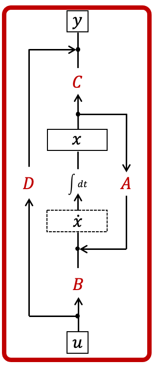
Typically, in our applications we'll learn $C$ as a transformation below, and we'll just set $D$ to a scalar multiple of the identity (or a residual connection, as we call it today).

1A: High-School Integral Calculus to Find $x$

With this ODE, we can write it directly in an integral form

Given input data and a value of $A$, we could in principle numerically integrate to find any value at any time $s$. This is one reason why numerical integration techniques (i.e., quadrature) are so important—but we have so much great theory, we can use them to understand what we're learning—more later.

Wake Up!

If that put you to sleep, wake up! Something amazing has already happened:

The term $\int_{0}^{s} e^{A(s-t)} B u(t) \; dt$ in Eqn. 1 is exactly of the form of a continuous-time convolution over the input data. Here's a visual demonstration:

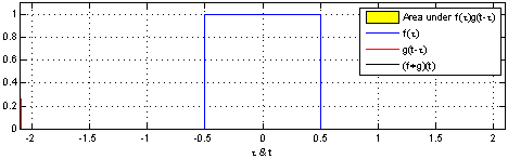
In our case, $Bu(t)$ is the equivalent of the blue signal $f(\tau)$ in the visualization, and $e^{A(s-t)}$ is the equivalent of the red convolution filter $g(t-\tau)$ in the visualization. So it seems intuitively clear we can use convolutions to estimate it. We’ll return to this in a moment, but we need to handle one bit of housekeeping.

1B: Samples of Continuous Functions: Continuous to Discrete

The housekeeping issue is that we don't get the input as a continuous signal. Instead, we obtain a sample of the signal of $u$ at various times, typically at some sampling frequency $T$, and we write:

That is, we use square brackets to denote the samples from $u$ and similarly the sample from $x$ as well. This is a key point, and where many of the computational challenges come from: we need to represent a continuous object (the functions) as discrete objects in a computer. This is astonishingly well studied, with beautiful theory and results. We'll later show that you can view many of these different methods in a unified approach due to Trefethen and collaborators, but we expect this to be a rich connection for analyzing deep learning.

1C: Finding The Hidden States

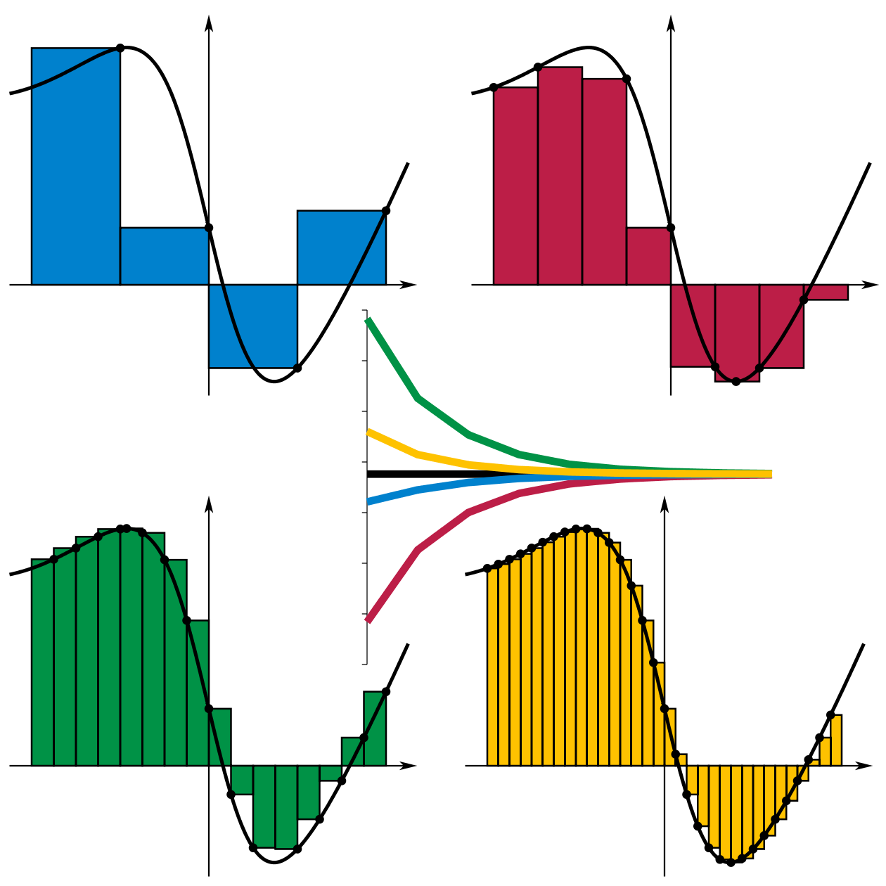
Recall that it's approximated by each rectangle using the left-end-point rule:

You may protest, and say, there are better rules than the left-hand-side rule for quadrature including the trapezoid rule, Simpson's rule, or Runge-Kutta! And yes, you'd be right! For now, we'll pick this rule because it's super simple. First, we rewrite Equation 1 slightly, factoring out $e^{As}$:

Then, for notational convenience, we define $g$, and we can compute it easily from $u$

Now, we can write

Now we have a really simple recurrence! We can compute it efficiently in the number of steps. This is a recurrent view, and we can use it to do fast inference like an RNN. Awesome!

1D: Convolutions

We want to push the $e^{As}$ inside the integral, which might be less prone to overflow—and it makes the connection to convolutions more clear. Let $f[k] = Bu[k]$ and $h[k] = e^{AkT}$ then for each value of $k$ define:

Recall from Eqn. 1, that we approximate using our rectangle rule:

And so

Now two comments: You could implement this with a typical convolution in pytorch, but those are optimized for small kernels (think $3 \times 3$ kernels). Here the convolution is of two long sequences, and so we use the standard FFT way of doing a convolution. However, much more important is a subtlety with batching that can make us much faster — by never materializing the hidden state $(x[k])$.

Part 2: From Control Systems to Deep Learning

How do we apply this to deep learning? We'll build a new layer which is effectively a drop-in replacement for attention. Our goal will be to learn the $A, B, C$, matrices in the formulation. We want this process to be a) stable, b) efficient, and c) highly expressive. We'll take these in turn—but as we'll see they all have to do with the eigenvalues of $A$. In contrast, these properties are really difficult to understand for attention and took years of trial and error by a huge number of brilliant people. In S4, we're leveraging a bunch of brilliant people who worked this out while making satellites and cell phones.

2A: Stable

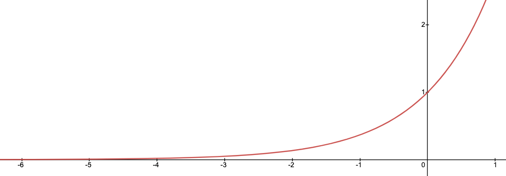
One thing that every electrical engineer knows is "keep your roots on the left-hand side of the plane." They may not know why they know it, but they know it. In our case, those roots are the same as the eigenvalues of $A$ (if you're an electrical engineer, they actually are the roots of what's called the transfer function, which is the Laplace transform of our differential equation). If you're not an electrical engineer, this condition is for a pragmatic, simple reason. Recall that for a complex number $\lambda$:

So if $\lambda$ is in the left-hand side of the plane, i.e. $\mathsf{real}(\lambda) < 0$, then the value does not blow up to infinity! In our case, $\lim_{n \to \infty} e^{ATn}x(0)$ could spiral off to infinity, if even one eigenvalue of $A$ were on the right hand side (with higher real part). This is related to what's called Bounded-Input, Bounded-Output (BIBO) stability—and there are many more useful notions, those signal processing folks are smart! Read their stuff! For us, it gives us a guideline—our matrix $A$ better have its eigenvalues on the left-hand side of the plane! We observed this was absolutely critical in audio generation in Sashimi, which let us generate tons of creepy sounding audio. There we use the so-called Ruth-Hurwitz property, which says the same thing.

2B: Efficient

We'll give two observations. First, as we'll see, for a powerful reason it suffices to consider diagonal matrices. This simplifies the presentation, but it's not essential to scalability—in fact, Hippo showed you could do this for many non-diagonal matrices. Second, we'll show how to compute the output $(y[k])$ without materializing the the hidden state ($x[k]$), which will make us much faster when we do batched learning. The speed up is linear in the size of the batch—this makes a huge difference in training time!

Diagonal Matrices

Here, we make a pair of observations that almost help us:

• If $A$ were symmetric, then $A$ would have a full set of real-valued eigenvalues, and it could be diagonalized by a linear (orthogonal) transformation.
• Since this module is a drop-in replacement for attention, the inputs (and the output) are multiplied by fully-connected layers. These models are capable of learning any change of basis transformation.

Combining these two observations, we could let $A$ be real diagonal matrices and let the fully connected layer learn the basis—which would be super fast! We tried this, and it didn't work... so why not?

We learned that to obtain high quality the $A$ matrix often had to be non-symmetric (non-hermitian) — so it didn't have real eigenvalues. At first blush, this seems to mean that we need to learn a general representation for $A$, but all is not lost. Something slightly weaker holds:

This is related to the fact that simple polynomials like $p(x)= x^2 + 1$ do not factor over the real numbers but any polynomial factors completely over the complex numbers into linear terms, here $p(x)=(x+i)(x-i)$. We link to the proof of more subtle, formal versions of this statement, which use phases like "measure one" if they are familiar to you. For deep learning applications, this means:

This is a great simplification—no fancy matrix exponentials. This was nicely empirically observed in (Gupta et al. 2022) without the explanation above and with more detailed description. Note that S4 can be efficient and stable even if you don't assume it's diagonal, but the math gets a little more complex.

So now letting $\lambda_i$ be our complex, unordered eigenvalues we can think about the far simpler set of $d$ one-dimensional systems:

We can again compute this using our rectangle or convolution method—and life is good!

Even Faster! No Hidden State!

In many of our applications, we don't care about the hidden state—we just want the output of the layer, which recall is given by the state space equation:

In examples, $y(t)$ is much lower dimensional than $x(t)$. For example, $y(t) \in \R$, while the hidden state is often much larger in $x(t) \in R^{d}$, where $d = 64$. If we could avoid materializing $x$, we could potentially go much faster. For simplicity of notation, set $x(0) = 0$ and $D = 0$ (typically we'll just use $D = I$ following our pioneering vision friends with residual connection). In this setup, we compute:

Importantly, we hope to never materialize $x(s)$ — so we have to be clever with the term $Ce^{A(s-t)}B$ since naively it's as big as $x(s)$.

Conjugate Pairs The key term is $Ce^{A(s-t)}B$, and we'll use a key property of it: it's real for any value of $t$. $C \in R^{1 \times d}$ and $B \in \R^{d \times 1}$ so we'll just use vectors $c$ and $b$. We want to use the diagonal formulation above and so with this simplified notation we have:

This holds for all values of $c_1,b_1, c_2, b_2$ for any valid choice of $\lambda_j$.

If we set $\lambda_j$ to arbitrary complex numbers, this may no longer be real. Indeed, since $A$ is real and its eigenvalues have more structure, its eigenvalues come in conjugate pairs: if $\lambda$ is an eigenvalue, so is $\bar \lambda$. We zoom in on a pair of these to derive a sufficient condition to keep the entire term purely real:

Since a complex value is real if and only if $x$ is equal to its complex conjugate, i.e., $x = \bar x$, we have

Thus, we'll only store half of the conjugate pairs since we'll ``tie'' the parameters of the other conjugate pair.

Thus, our equation can be written:

Below, we'll cheat a bit and call $d/2$ as $d$ from now on, since it's nicer to look at.

Saving the Kernel: Big Batch Training One advantage of this setup is that we only need to compute the kernel once, which is of size $n$ instead of size $n \times d$. To create it will take $O(nd)$ time and space, but when we use it on a batch of size $b$, we can save a large factor. Roughly, our algorithm will run in time $\theta(nd + bn)$ — rather than $\theta(bnd)$.

To see how, return to our equation:

Noticing that $e^{\lambda} + e^{\bar \lambda} = 2 e^{a}\cos(\theta)$ where $\lambda = e^{a + \theta i}$. We simplify one more time:

This step is nice because it means we got rid of the complex values! Now, to write this as a convolutional form with the rectangle rule, we define:

Then, following Eqn. 2, we can write $y[k]$ as the convolution (recall $T$ is the sampling frequency).

Notice that we can compute $f$ above, once per batch. In particular, $f \in \R^{n}$ and as claimed we use $O(nd)$ time and memory to construct it. When we have batches, instead of $g \in \R^{n}$ in our simplified example, we have $g \in R^{b \times n}$ for some batch size $b$. If we performed the operation naively, we could potentially create an object of size $b \times n \times d$ — and a runtime of $\Omega(nbd)$ — but instead we refactor into $(f,g)$ as above, so our running time and memory is in $O(n(d + b))$.

Bringing Back the Initial Condition Recall Eqn. 3, we want to add back the $x[0]$ initial condition. This means we should compute:

That's it! We add that in at each time step. Note if we choose to fix $x[0]=0$, then we could combine $c_j$ and $b_j$ into a single value, i.e., $q_j = c_jb_j$. We show this optimization in the code.

Code Snippet These optimizations lead to a very concise forward pass (being a little imprecise about the shapes):

l : int  = u.size(-1) 
T : int  = 1/(l-1)    # step size
zk : Tensor        = T*torch.arange(u.size(-1))
base_term : Tensor = 2*T*torch.exp(-self.a.abs() * zk) * torch.cos(self.theta * zk)
q : Tensor  = self.b*self.c         
f : Tensor  = (q*base_term).sum(-1)
y : Tensor  = conv(u,f)

2C: Highly-Expressive Initialization

Forgetting is Critical We examine a single term from Equation 4 (dropping the $j$) to emphasize the key quantities:

Recall that $n$ is the length of the sequence (and $T=n^{-1}$), and $\delta$ is the number of samples between the values of $s-t$. As engineer's intuition, if $|a| \delta < 5n$, then this term is effectively $0$ (namely it's smaller than $e^{-5}\approx 0.006$):

That is, $a$ is inversely proportional to how many steps this SSM can possibly remember. In particular, if $n=1024$ and $a = -128$ this would mean that we could remember about $n/a \approx 40$ steps. While if $a=0$ then the SSM can (in principle) learn from the entire sequence—but it may be using stale or irrelevant information. Ideally, we'd like both modes—and a few in between!

SSMs at Multiple Scales Inspired by our convolutional friends, we typically learn multiple SSMs from each sequence, say $h$ different copies. Following the intuition above, we initialize these SSMs at a variety of different scales using a simple geometric initialization. For concreteness, suppose the sequence length is $n=1024$. Let $a_{i,j}$ be the $i=1,\dots,h$ be the index of the SSM and $j$ be the component of that SSM. Then, our proposed initialization is:

The Frequency Component The motivation for the initialization of $\theta$—which doesn't depend on $h$—is that we simply we want the integer frequencies. A bit deeper connection is that there is a very famous sequence of orthogonal polynomials, called the Chebyshev polynomials that pop up everywhere. In part, the reason for their seeming ubiquity is that they are extremal for many properties, e.g., they are the basis that has the minimal worst-case reconstruction error—and are within a factor of two. (In a follow-on post, we will walk about these connections in more detail. These polynomials are defined by the property $t_k(\cos \theta) = \cos(k \theta)$:

Thus, choosing $k$ in this way effectively defines a decent basis.

For both of these, there are surely more clever things to do, but it seems to work ok!

Wrapping Up

Now that we've gone over the derivation, you can see it in action here. The entire kernel takes less than 100 lines of PyTorch code (even with some extra functionality from the Appendix that we haven't covered yet).

We saw that applying LTI systems to deep learning, we were able to use this theory to understand how to make these models stable, efficient, and expressive. One interesting aspect of these systems we inherent is that they are continuous systems that are discretized. This is really natural in physical systems, but hasn't been typical in machine learning until recently. We think this could open up a huge number of possibilities in machine learning. There are many improvements people have made in signal processing to discretize more faithfully, handle noise, and deal with structure. Perhaps those will be equally amazing in deep learning applications! We hope so.

We didn't cover some important standard extensions from our transformer and convolutional models—it's a drop in replacement for these models. This is totally standard stuff, and we include it just so you can get OK results.

• Many Filters, heads or SSMs: We don't train a single SSM per layer—we often train many more (say 256 of them). This is analogous to heads in attention or filters in convolutions.
• Nonlinearities: As is typical in both models, we have a non-linear fully connected layer (an FFN) that is responsible for mixing the features—note that it operates across filters—but not across the sequence length because that would be too expensive in many of our intended applications.

Further Reading If you like this blog post, here are some great resources to go further!

• The Annotated S4
• S4 Paper
• SaShiMi
• S4D

Acknowledgments Thanks to Sabri Eyuboglu, Vishnu Sarukkai, and Nimit Sohoni for feedback on early versions of this blog post.

Appendix: Signal Processing Zero-Order Hold

In signal-processing, a common assumption on signals (made in the S4 paper, and its predecessor Hippo) is called "zero-order hold." The zero-order hold assumption is that the signal we're sampling is constant between each sample point, or in symbols: $u(k+\delta) = u[k]$ for $\delta \in [0,T)$. This changes the approximation—but only by a small amount. This appendix describes the difference. Namely, we will show that:

in which $f[k] = e^{ATk}$ and $g[k] = Bu[k]$. Note this is exactly the same as the convolution from Equation 3.

Derivation For context, we previously used the following approximation

Using the zero-order hold assumption, we have the following:

We can compute this integral exactly:

For notation, let $Q = A^{-1}\left(I-e^{-AT}\right)$ Just as above, we have a recurrence:

Convolution We can also exactly relate the sum to the same convolution from Equation 3:

in which $f[k] = e^{ATk}$ and $g[k] = Bu[k].$

Diagonal Case In the diagonal case,

Here, we get essentially the same convolution with a different constant.

Comparison with the Other We compare this to the block integration:

Typically, $T=1/n$ where $n$ is the sequence length. Hence, if the eigenvalue $\lambda$ is $o(n)$, then this will be essentially $T$, which matches the previous section. For very large eigenvalues, it becomes more different.

Removing Hidden State When we remove the state, this doesn't seem to simplify quite as nicely. We need to group the expression for $\lambda$ and $\bar \lambda$.

Thus, if we define $f_j[k] = h(\lambda_j, k) + h(\bar \lambda_j, k)$ and $g_j[k] = u_j[k]$. Then,