Dec 1, 2025 · 28 min read
Our In-House Recipe for Juicy, Fact-Stuffed MLPs
Owen Dugan*, Roberto Garcia*, Ronny Junkins*, Jerry Liu*, Chris Ré
TL;DR (click to expand):
Transformers store much of their factual knowledge inside MLP layers, but how they do it is still unclear. Whereas most previous efforts to understand MLP fact storage have focused on probing trained LLMs, we take a generative approach: we explicitly construct MLPs that implement key-value fact mappings. This gives us provable guarantees of correctness, precise facts-per-parameter scaling laws, and new insights into how embedding geometry affects MLP parameter efficiency and how transformers can reliably use MLPs. Our construction is the first to be:
- Provably Efficient: for some embeddings, our construction matches the information-theoretic limit of bits to store facts.
- General: our construction handles realistic, non-uniform embeddings.
- Usable: Transformers can learn to use our MLPs for factual recall.
In this blog, we'll dig into the details of our construction.
In Part 1, we introduced our generative view of factual recall in MLPs. Here, we zoom in on the construction: we'll explain how to turn a set of key/value embeddings into a provably correct and efficient fact-storing MLP. We’ll keep the math light and focus on the core intuitions throughout.
The Hazy Research Lab Cooking Juicy, Fact-Stuffed MLPs!
Problem setup
First, let’s formalize what it means for an MLP to store a set of facts.
We're given key embeddings , value embeddings , and a fact map that assigns each key its correct value.
We'll say that an MLP stores this fact set if, for every key , its output is closer (under dot-product decoding) to the correct value than to any other:
We use the dot product as our similarity measure because it matches the softmax decoding used in language models; this is also the same setup used in prior work.
We quantify our construction's parameter efficiency via its fact-storage cost: we define this as the minimum number of parameters a model family needs to represent every possible fact map over . (Lower is better!)
A simple counting argument gives us a lower-bound on fact-storage cost, assuming constant bits per parameter: any model family must use at least
parameters. Intuitively, there are possible mappings from keys to values, so just identifying which mapping you want already takes bits.
In this blog, we'll focus on using gated MLPs to store facts. Particularly, we'll consider MLPs of the form
where is any activation function (we focus on ReGLU or SwiGLU MLPs in this blog). Check out the paper for more details on non-gated MLPs!
Our goals
With the basic setup in place, we can now spell out what we want from our constructed MLPs. Compared to prior constructions, our approach is designed to achieve three goals:
-
Handle general embeddings.
Prior work focuses on key and value embeddings that are uniformly spherically distributed, but embeddings from language models are anisotropic and structured. We'll provide a construction that works for all but a measure-zero set of feasible embeddings (those with , as described below). -
Match our information-theoretic baseline.
Ideally, our constructed MLPs should match the baseline of parameters. We'll show that our construction matches this baseline up to a geometry-dependent constant:where is a decodability factor we introduce shortly. For "well-spread" embeddings such as spherical ones, , giving a scaling of . This scaling asymptotically matches the parameter count of our information-theoretic baseline and requires a factor of fewer parameters than the lowest bound from prior work.
-
Be usable inside Transformers.
We want Transformers to be able to use our constructed MLPs for factual recall, with fact-storage cost that scales similarly to the MLP's fact-storage cost. Our construction handles this too, but we'll leave the details for Part 1 of our blog post.
Here, we'll focus on the first two goals.
Roadmap
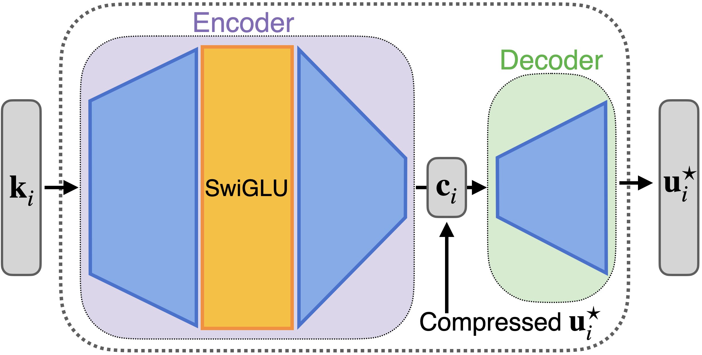
We factor the MLP into a gated encoder and a linear decoder to achieve asymptotically optimal scaling.
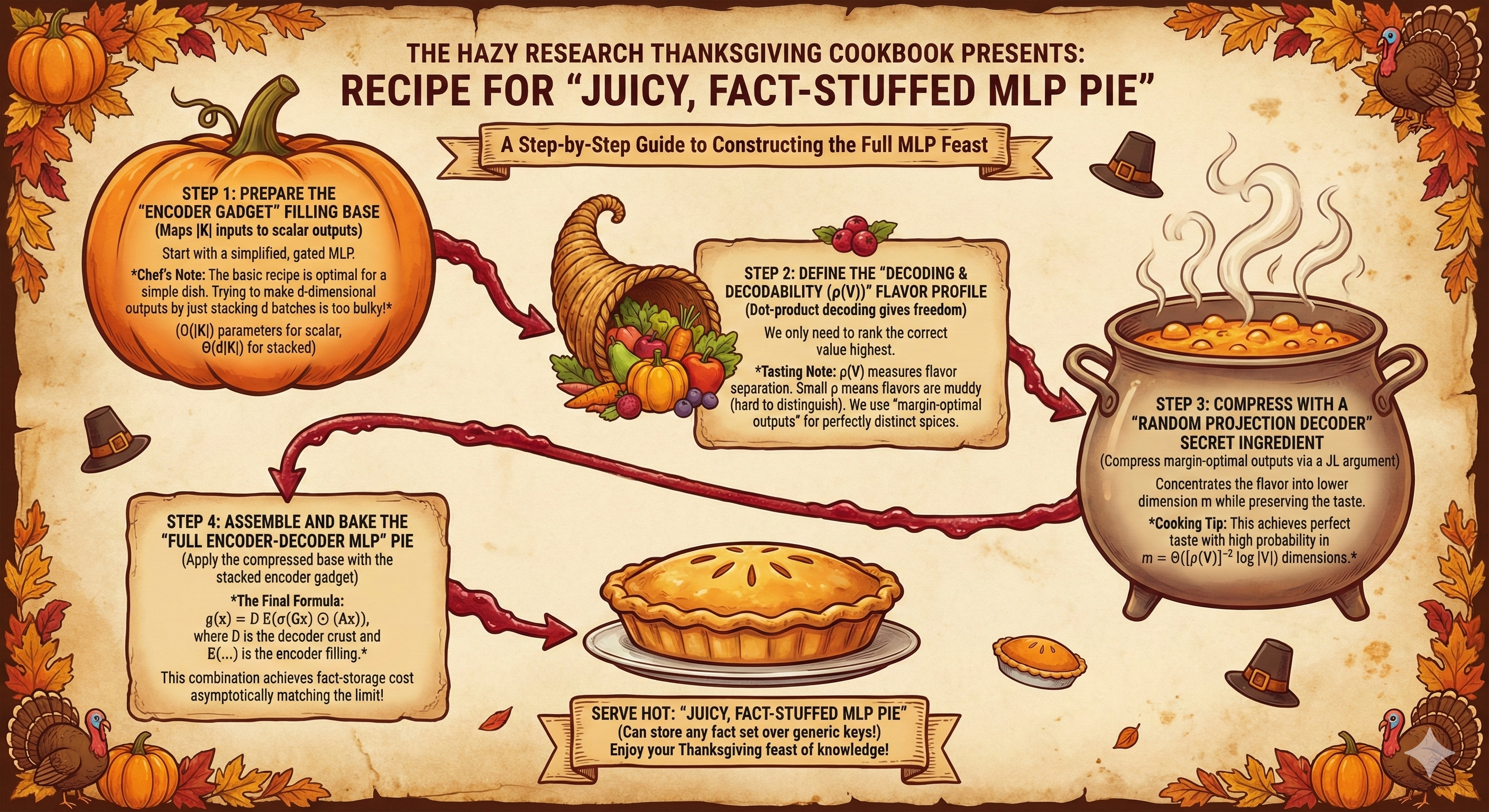
We’re now ready to walk through the main ideas behind the construction. We’ll build up to the full MLP in a few steps:
-
Encoder gadget.
We start with a simplified setting and construct a gated MLP that maps inputs in to arbitrary scalar outputs using only parameters. This “encoder gadget” is essentially optimal (up to a constant factor) for the scalar-output case. However, naïvely stacking copies of this gadget to produce -dimensional outputs still requires parameters, which is too large to achieve our target scaling. -
Decoding and .
Dot-product decoding gives us an extra degree of freedom: our MLP doesn’t need to output the value embeddings themselves, only vectors that rank the correct value highest under dot-product similarity. This leads us to the decodability , which measures how geometrically "separated" the value embeddings are. Small means the values are tightly packed and require more parameters to separate; large means they’re easier to distinguish. To take advantage of this, we introduce margin-optimal outputs, a set of output vectors that can maximally distinguish each value embedding from all other value embeddings. -
Compression via a random projection decoder.
The final idea to achieve our target scaling is to compress the margin-optimal outputs to a lower-dimensional code while preserving the dot-product decoding constraints. We show that a simple random linear projection suffices via a Johnson–Lindenstrauss (JL) argument. With this choice of decoder, projecting intodimensions achieves perfect decoding accuracy with high probability.
-
Full encoder-decoder MLP.
The exponential reduction in output dimension from compression now lets us directly apply our stacked encoder gadget and, for many embeddings, allows us to achieve fact-storage cost asymptotically matching our information-theoretic baseline! This yields our final construction:where is the JL-style decoder and is the encoder. We show our construction can store any fact set over generic keys and decodable values with fact-storage cost
Our encoder gadget
We first focus on a simplified setting:
Can we construct a gated MLP that maps a finite set of inputs in to arbitrary real numbers, using only parameters for datapoints?
Our plan is to stack multiple copies of this encoder gadget to produce full outputs.
We’ll start with a particularly nice choice of key embeddings as a warmup: two-hot difference vectors of standard basis vectors.
A toy setting: two-hot differences
Fix a dimension and consider the set of inputs
which has elements. For each ordered pair with , we choose an arbitrary target scalar .
Our goal is to build an MLP such that
The encoder gadget construction
In this setting, we propose a simple weight construction for a 1-hidden-layer gated MLP, which we call our "encoder gadget":
where
Intuitively, constructing the encoder gadget has two steps: 1) pick a gating term to cause different hidden neurons to select different "portions" of the inputs, then 2) set the matrix so it fits the data.
How does this work?
Plugging in a two-hot input with :
-
Gating step.
since has a in coordinate and a in coordinate (which gets zeroed out).
-
Linear step.
The -th coordinate of this vector is
-
Elementwise product + sum.
Gating zeroes out all but the -th coordinate:Summing with gives the scalar .
From toy to general embeddings
The two-step core idea behind the encoder gadget extends beyond the two-hot embeddings setting:
- Instead of using the identity as the gating matrix, we choose a more general gating matrix . For analytic activation functions like Swish/SwiGLU and GeLU/GeGLU, our construction works for generic (for all but a measure 0 set of possible ), so we can just sample a random matrix with i.i.d. Gaussian entries.
- Once the gating matrix is fixed, the network becomes linear in the remaining weights. This means we can solve a linear system to find an matrix that matches any desired outputs.
The encoder gadget recipe for general embeddings:
Fix a generic . For each key , the encoder gadget produces
so each encoder output is a linear function of .
Stacking these equations for all and all gives a single linear system of the form
where:
- is just all the entries of flattened,
- contains the desired outputs , and
- depends only on the keys and the gating terms .
In the paper, we show that the construction holds for generic with enough rows (roughly ), for commonly-used activation functions like GeLU and Swish (and more generally any non-polynomial analytic function), for all but a measure-zero set of key embeddings, and for all choices of target scalars. For example, with Swish gate activations, our construction produces SwiGLU MLPs, like those from modern frontier models (e.g., Llama or Qwen).
Encoder Construction (sketch)
- Choose a generic gating matrix .
- Compute the gating vectors for all keys.
- Form and solve the resulting linear system to find such that for every .
Parameter count.
A simple degrees-of-freedom argument shows that we need at least parameters to specify arbitrary outputs on inputs. When , our encoder uses
parameters: one set of parameters for , one for , and minor overhead for the readout. For , this stays within a constant factor of the lower bound.
Our first construction attempt (and why it’s not enough)
Our encoder gadget already gives us a simple way to solve the full problem.
If the gadget lets us map from , then to map from we can just stack copies of the gadget — one per output coordinate!
Excitingly, this naïve construction is provably correct, and already works for a broader range of inputs/outputs than prior constructions! However, it uses parameters, which can be much larger than our information-theoretic
bound when (e.g., for typical LLM embedding dimensions).
To do better, we need to take advantage of our decoding mechanism.
Exploiting dot-product decoding
Let’s step back and look at the dot-product decoding condition again. For a fact set , we require
A simple observation:
We don’t need to equal ! We only need it to rank the correct value with the largest dot-product score.
This leads to two key ideas:
- We should pick MLP outputs that maximize the decoding margin — and they don't necessarily need to equal .
- We can compress these output embeddings into a lower-dimensional space, as long as the inequalities hold after decompression.
Decodability
To motivate the first idea, we ask a simple question: how hard is it to tell the value embeddings apart using dot-product decoding? Some sets of value vectors are easy to distinguish; others are tightly clustered and require much larger margins to separate. We capture this with a single geometric quantity, the decodability .
Intuitively, measures the best achievable margin between each value and all competing values under dot-product decoding. Larger means the values are well-separated and easy to decode; smaller means they’re packed together and require more parameters to separate.
Before we define , we note that it turns out to be a fundamental quantity for fact-storing MLPs. For , there are no MLPs that can store certain fact sets over . Additionally, is predictive of fact-storage cost (equivalently, MLP size) across gradient-descent-trained and constructed MLPs (both ours and from prior work (NTK)!).

Fact-storage cost depends on the decodability of the output embeddings.
Now, let's define . Formally,
This is the largest worst-case (normalized) margin we can give every value by choosing appropriate output vectors .
Given our definition of , a natural choice of MLP output is to take, for each value, the margin-optimal output direction
is the spherical Chebyshev center of the vectors (for ) — geometrically, it's the direction that most robustly separates from all other values. Our paper contains a more detailed justification of . Here we'll simply foreshadow that turns out to be the optimal output for our decoder.
Compressing margin-optimal outputs
The second key idea is to use compression to reduce the dimension of the MLP outputs. Conveniently, dot-product decoding only depends on the sign of certain inner products:
If we can compress and decompress the while preserving these signs, decoding will still work.
Our decoder stems from the following observation: a Johnson–Lindenstrauss–style random linear projection with
is enough to keep all the relevant inner-product signs intact with high probability.
Why does this work?
After compression,
and decoding depends only on the sign of
Random projections preserve all pairwise inner products up to a small (less than ) distortion when
Since the original inner products have a margin of at least , distortions smaller than cannot flip the signs. This means that decoding continues to work after compression!
Decoder Construction (sketch)
- Start with the margin-optimal outputs .
- Sample a random projection matrix (e.g., i.i.d. Gaussian).
- Form compressed codes
- Decode by projecting back up:
Then , and the decoding inequalities are preserved.
The key insight: now that we can reduce the output dimension from to using our decoder, we can revisit our stacked-encoder idea and finally make it parameter-efficient!
Putting everything together: the full construction
Let's combine the encoder and decoder into a single MLP that stores an arbitrary fact set over generic keys and decodable values. The resulting model has the form
where form the encoder, is the decoder, and is a gating activation function (e.g., ReLU, GeLU, Swish). The encoder produces a compressed code in ; the decoder maps it back into so that the output dot-product-decodes to the correct value embedding.
To see our full recipe:
Our MLP Construction (sketch)
Choose compressed outputs.
Compute margin-optimal outputs and draw a random projectionForm compressed codes
Construct the encoder.
Treat as the target outputs and use the encoder to find weights
such thatAssemble the full model.
Our main theoretical result shows that our proposed construction satisfies our goals of asymptotic scaling and generality:
Theorem (Full construction, informal).
For any fact set , generic keys , and values with , the above construction yields a fact MLP that stores and has fact-storage cost
For value embeddings with , such as uniformly-spherical embeddings, this matches our information-theoretic baseline of , improving over bounds from prior work by a factor of .
Since we have matched the parameter count asymptotics of our information-theoretic baseline, we can next ask how many bits per parameter our construction uses. For the two-hot example, we actually achieve a constant number of bits per parameter (leading to information-theoretically optimal scaling in the total number of MLP bits), and, for embeddings such as the uniform spherical embeddings assumed by prior constructions, our construction uses bits per parameter. In both cases, our construction comes within a single log factor of the information-theoretically optimal rate, when measured in bits.
Table 1 summarizes how our construction compares to bounds on prior fact-storing MLP constructions.
| Construction | Parameters | Hidden Sizes | Assumptions on | Assumptions on |
|---|---|---|---|---|
| Info-theoretic Baseline | None | None | ||
| Naïve (stacked encoder gadgets) | Generic | |||
| Nichani et al. (2024) | Uniform on | Uniform on | ||
| Ours | Generic |
How close are we to optimal in practice?
So far we’ve focused on theory; how well does the construction work empirically?
To test this, we compare several MLP families. We compare our construction (which we label "Ours: Bin + JL") against the following baselines:
- GD MLPs: fully end-to-end MLPs trained directly on the dot-product decoding objective using gradient descent and a cross entropy loss
- NTK MLPs: the construction from Nichani et al. (2024)
In addition to the GD and NTK baselines, we evaluate ablations of our encoder-decoder framework:
-
GD encoder (Ours: GD + JL):
We keep the JL decoder fixed, but instead of using the explicit encoder gadget, we train the encoder parameters with gradient descent and a mean-squared-error loss so thatfor the target compressed codes .
-
GD decoder (Ours: Bin + GD):
We keep the encoder gadget fixed, but instead of using a random projection as the decoder, we train a linear map and compressed codes with gradient descent and a cross entropy loss on the logits -
GD encoder + GD decoder (Ours: GD + GD):
We keep the same encoder-decoder architecture as our construction, but with both the encoder and decoder parameters learned with gradient descent. The encoder and decoder are trained separately.
We fix the embedding dimension (), sample uniform-spherical embeddings, and vary the number of facts. For each MLP family, we measure the minimum number of parameters needed to perfectly store a randomly chosen fact set.
Three observations stand out:
-
Our MLPs match GD MLPs' asymptotics.
The explicit construction (Bin + JL) follows the same asymptotic trend as GD-trained MLPs as the number of facts grows. In contrast, NTK MLPs exhibit asymptotically worse scaling with increasing number of facts and fixed embedding dimension. -
We consistently outperform NTK.
Even in this clean spherical setting, our explicit MLP is roughly more parameter-efficient than NTK-based constructions — and the gap widens with more facts. Around facts, NTK MLPs fail to achieve perfect fact storage while ours continue working. -
Our encoder-framework is performant when partially learned.
Using a GD-trained encoder together with a GD-trained decoder gets us most of the way to the parameter-efficiency of fully gradient-descent-trained MLPs (worse by , better than NTK by ). This suggests that our encoder-decoder framework captures most of the structure that gradient descent discovers.
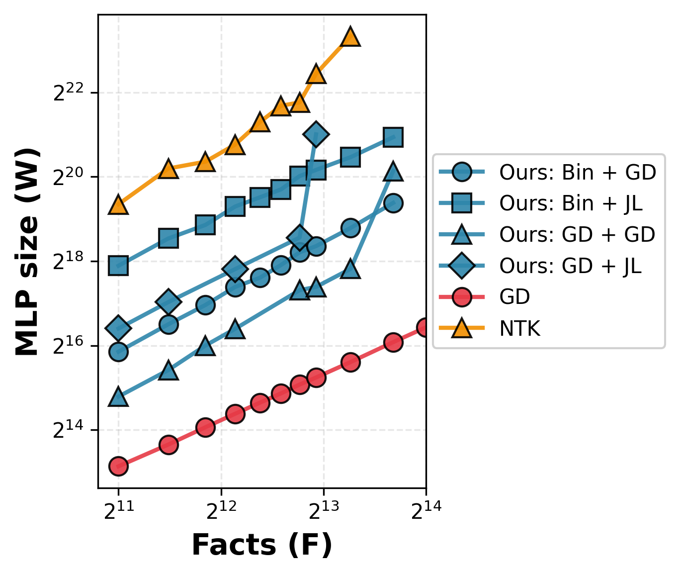
Our explicit construction (Bin + JL) matches the fact-storage scaling of GD-trained MLPs — and is asymptotically more parameter-efficient than prior constructions for large numbers of facts.
Conclusion
The Hazy Research Recipe for Juicy, Fact-Stuffed MLPs!
Acknowledgements
Thank you to Yasa Baig, Kelly Buchanan, Sam Buchanan, Catherine Deng, Andy Dimnaku, Junmiao Hu, Herman Brunborg, Rajat Dwaraknath, Jonas De Schouwer, and Atri Rudra for helpful feedback on this blog post.