Jul 7, 2025 · 13 min read
BWLer 🎳 (Part 2): Navigating a Precision-Conditioning Tradeoff for PINNs
TL;DR (click to expand):
Physics-informed neural networks (PINNs) offer a flexible, mesh-free way to solve PDEs, but standard architectures struggle with precision. Even on simpler interpolation tasks, without the challenging PDE constraints, we find multi-layer perceptrons (MLPs) consistently plateau at RMSE, far from float64's machine precision (around ). We introduce BWLer, a drop-in replacement for neural networks that models the PDE solution as a barycentric polynomial interpolant. BWLer can either augment a neural network (BWLer-hat) or fully replace it (explicit BWLer), cleanly separating function representation from derivative computation. This lets us disentangle precision bottlenecks caused by MLPs from those due to PDE conditioning. Across three benchmark PDEs, BWLer-hatted MLPs reduce RMSE by up to over standard MLPs. Explicit BWLer models can do even better — reaching RMSE, up to 10 billion times improvement over standard MLPs — but they require heavier-duty, second-order optimizers. BWLer exposes a fundamental precision–conditioning tradeoff, and gives us tools to navigate it — one step toward building precise, flexible, and scalable scientific ML systems.
⏮️ Part 1 of the blog post
📄 Paper
💻 GitHub
Full team: Jerry Liu, Yasa Baig, Denise Hui Jean Lee, Rajat Vadiraj Dwaraknath, Atri Rudra, Chris Ré
Corresponding author*: jwl50@stanford.edu

In Part 1 of this two-part blog post, we introduced the physics-informed framework and motivated the need for better, high-precision architectures — leading to BWLer (Barycentric Weight Layer). In Part 2, we'll dive deeper into how BWLer works, show how it achieves high-precision PDE solutions, and share what we're excited to explore next.
🎳 BWLer: Spectral interpolation meets deep learning
BWLer enhances or replaces the physics-informed neural network (PINN) with a high-precision polynomial. Instead of learning a black-box function that approximates the PDE solution everywhere, we define the solution globally using a barycentric polynomial interpolant — a classical tool from numerical analysis known for its stability and spectral accuracy.
The idea is simple: rather than using a neural network to represent the solution across the domain, we fix a grid of interpolation nodes and represent the solution entirely by its values at those nodes. BWLer then interpolates the solution using a closed-form formula, and computes derivatives using efficient spectral methods. The model remains fully differentiable and can be trained with standard ML optimizers like Adam.
BWLer supports two modes (see Figure 1):
- In a BWLer-hatted MLP, the MLP predicts the node values, and BWLer handles interpolation and differentiation downstream.
- In explicit BWLer, we discard the MLP entirely and directly optimize the node values as parameters.
By separating representation from differentiation, BWLer exposes new knobs for controlling precision and numerical conditioning — while remaining fully compatible with the physics-informed training.
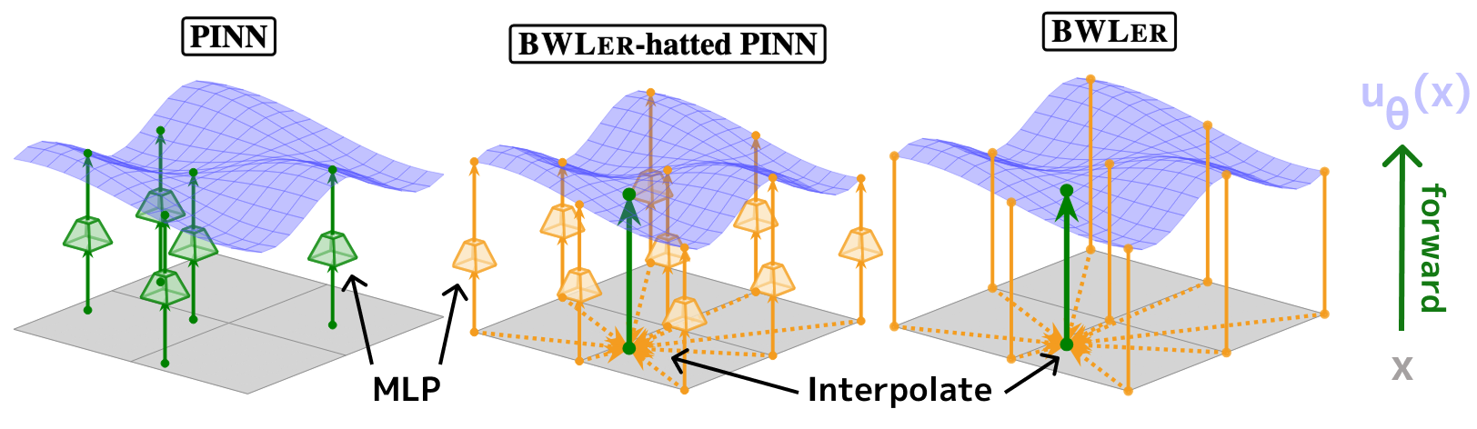
Figure 1: Standard PINNs evaluate a neural network everywhere. BWLer defines a solution globally using interpolation at a fixed grid of nodes.
If you're interested: how BWLer works under the hood
BWLer uses barycentric Lagrange interpolation, specifically the second barycentric formula:
Here, are interpolation nodes, are the function values at those nodes, and are precomputed barycentric weights. When the nodes are well-chosen (e.g. Chebyshev nodes), this formula is stable and accurate even for high-degree polynomials, and requires no explicit basis functions.
To compute PDE losses, BWLer differentiates the interpolant using:
- Spectral derivatives, such as FFTs or Chebyshev differentiation matrices.
- Or finite-difference approximations, when better conditioning is needed.
All operations remain fully differentiable with respect to the node values , so BWLer integrates seamlessly into any physics-informed training loop.
🎩 BWLer-hatted PINNs: boosting precision with a single extra layer
Our first experiment with BWLer kept the neural network, but changed how we used it. Instead of evaluating the MLP everywhere in the domain and relying on autodiff to compute derivatives, we ask the MLP to predict the solution at a fixed grid of interpolation nodes. BWLer then takes over: it interpolates the solution across the domain and computes PDE residuals using spectral derivatives. This yields a BWLer-hatted PINN — same MLP, same optimizer, but with representation and differentiation now cleanly decoupled (see Figure 2).
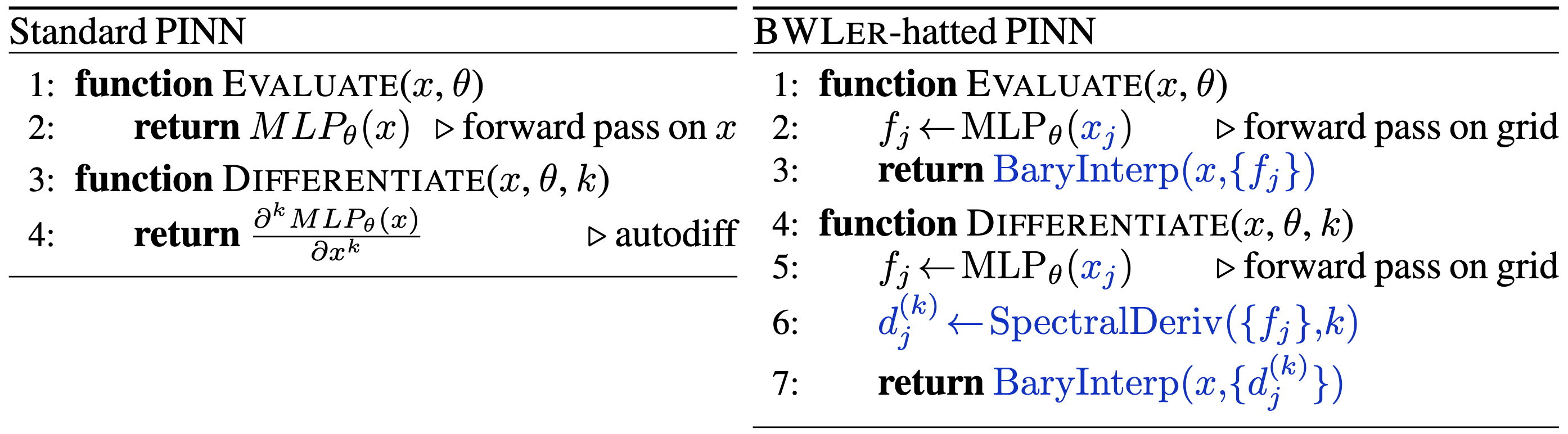
Figure 2: Standard PINN (left) vs. BWLer-hatted PINN (right). BWLer implements forward and derivative computations using spectral routines.
Importantly, this setup remains plug-and-play: you can drop BWLER on top of an existing PINN with minimal changes. But this extra polynomial layer leads to large improvements on smooth problems. Across three benchmark PDEs — convection, reaction, and wave equations — BWLer-hatted models reduce relative error by to compared to standard PINNs, with no extra supervision or architectural tuning.
Why does this work? BWLer-hatting imposes global structure in the way it treats the PDE. Unlike with standard MLPs, where derivative constraints are enforced locally, the interpolant's derivatives tie all points together, encouraging the network to learn globally coherent, smooth solutions. We find empirical support for the smoother convergence behavior: BWLer-hatted models consistently exhibit better-conditioned loss landscapes with lower Hessian eigenvalues.
| PDE | MLP | BWLer-hatted MLP |
|---|---|---|
| Convection | ( better) | |
| Reaction | ( better) | |
| Wave | ( better) |
Table 1: BWLer-hatted MLP improves precision (by -) on three benchmark PDEs.
🔬 Explicit BWLer: reaching machine precision by removing the neural network
As a proof of concept, we next took the BWLer approach one step further by fully decoupling function representation from derivative computation. In explicit BWLer, we treat the solution values at a fixed grid of interpolation nodes as directly learnable parameters. The model becomes a pure polynomial interpolant — a spectral approximation that’s fully differentiable and trained directly against the physics loss. No MLPs, no hidden layers; just node values and fast, precise derivatives.
This setup eliminates the representational limitations of neural networks and exposes the precision bottleneck sourcing from the poorly-conditioned PDE constraints. We find that we're able to push through these challenges using a heavier-duty, second-order optimizer (in our case, a method called Nyström-Newton-CG).
The results are striking. On the same benchmark PDEs, explicit BWLer achieves relative errors as low as , outperforming prior PINNs by up to in accuracy. As far as we know, these are some of the first PINN results to reach near machine precision, even on simple problems over 2D domains.
Crucially, we note that our results are not time- or parameter-matched comparisons! While explicit BWLer doesn’t yet match traditional solvers in runtime, our results show that machine-precision solutions are possible within the flexible physics-informed framework. We’re optimistic and excited about improving its efficiency and scaling it to more complex problems.
| PDE | Literature | Explicit BWLer |
|---|---|---|
| Convection () | (Rathore et al.) |
( better) |
| Convection () | (Wang et al.) |
( better) |
| Wave | (Rathore et al.) |
( better) |
| Reaction | (Rathore et al.) |
( better) |
Table 2: Explicit BWLer improves precision by up to 10 billion relative MSE on benchmark PDEs. Improvements are relative to the best published values (to our knowledge).
⚖️ The precision–conditioning tradeoff
Explicit BWLer unlocks a new regime of high precision, but it also surfaces a key tension at the heart of physics-informed learning: higher accuracy often comes at the cost of worse numerical conditioning.
Here’s the basic idea. Increasing the number of interpolation nodes makes the model more expressive and reduces approximation error, a hallmark of spectral methods. But there’s a catch: the resulting derivative matrices become more ill-conditioned, especially for high-order PDEs, which slows down optimization and can stall convergence. See Figure 3 for an example.
To understand this tension, we can break down total error into three components:
- Expressivity error: how well the interpolant can represent the true solution. Improves with more nodes.
- Bias error: how well the discretized PDE approximates the true one. Less accurate finite difference schemes introduce more bias than spectral derivatives.
- Optimization error: how close training gets to the best solution. Tied directly to how well-conditioned the loss landscape is.
These sources of error often pull in different directions. Spectral derivatives reduce bias but worsen conditioning. Finite differences improve conditioning but limit achievable precision by adding bias. Adding more nodes helps expressivity, but can worsen optimization if we aren't careful.
What makes BWLer useful here is that this tradeoff becomes explicit. We can swap in finite differences when needed, reduce node count, use heavier-duty optimizers like Nyström-Newton-CG, or warm-start from coarser solutions. These tools give us leverage to navigate the tradeoff in a controllable way, letting us push toward higher precision.
We suspect (and prior work suggests) that standard PINNs face a similar tradeoff — but they’re harder to reason about, because the MLP parameterization affects how derivatives for PDE constraints are computed. This may help explain why training techniques like curriculum learning or time marching work, and why so many optimization pathologies persist across the literature.
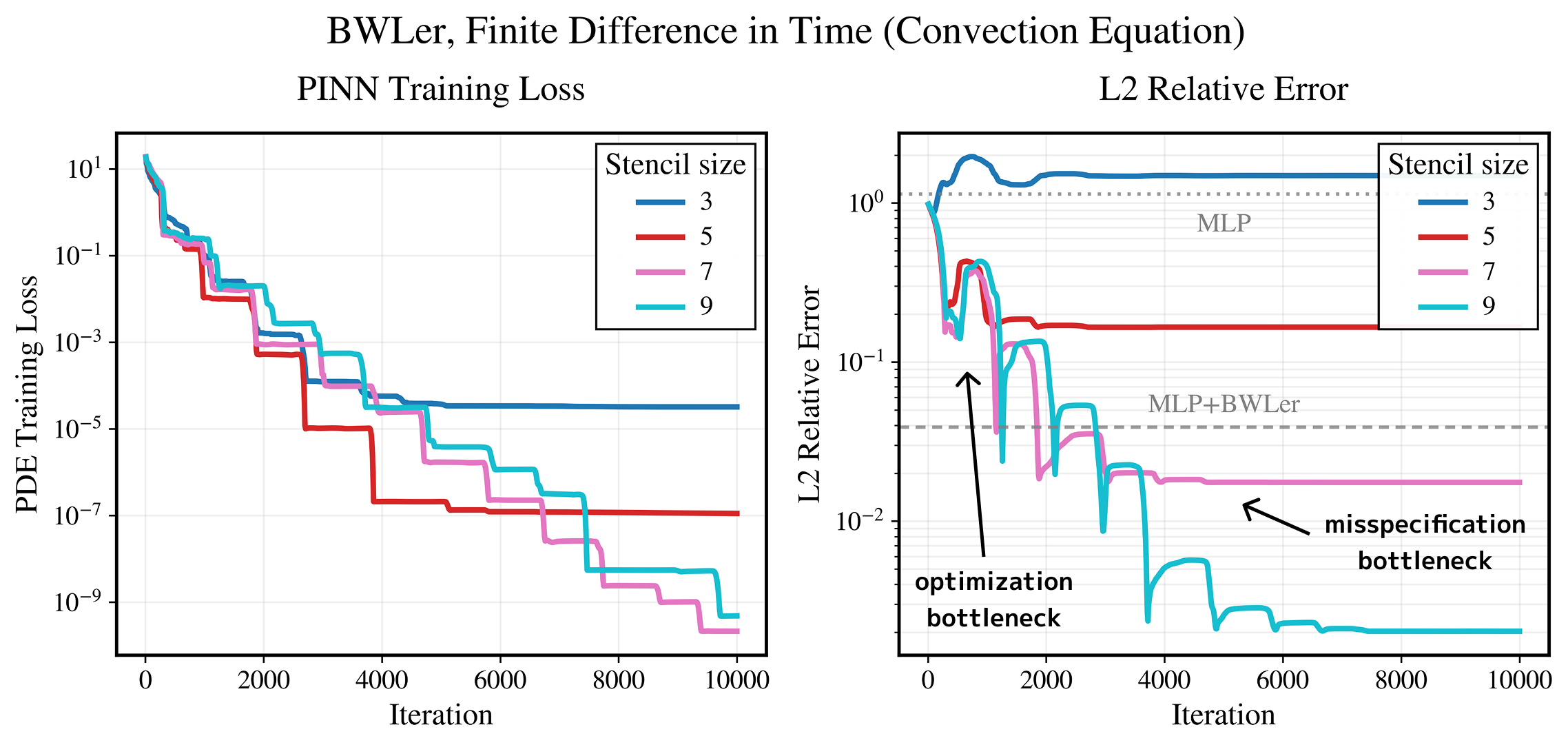
Figure 3: The precision–conditioning tradeoff becomes explicit with BWLer: finite differences improve conditioning (optimization) but adds bias (misspecification).
⚠️ Limitations of BWLer
While BWLer enables new levels of precision in scientific ML, it also inherits the known limitations of spectral methods. In particular, when the target solution exhibits discontinuities (e.g. PDEs for shock modeling) or is defined over irregular geometries, the PDE loss becomes significantly more ill-conditioned. We’re still able to match the precision of prior PINN results on these more difficult problems, but doing so requires heavier-duty optimization and much longer training times. For example, on Burgers’ equation and 2D Poisson, our current explicit BWLer setup required hours of wall-clock time to train, compared to just a few minutes for standard MLPs.
We view these results as a proof of concept — and just the beginning! One natural next step is a hybrid approach, where we start training with a rapidly-converging model (like a standard MLP) and switch to BWLer when higher precision is needed. We also suspect that many existing optimization techniques used to accelerate PINNs, like adaptive sampling or curriculum learning, could be repurposed to make BWLer more efficient.
See the paper for details, and stay tuned: we’re actively exploring ways to make BWLer more robust and efficient!
| PDE | Literature RMSE |
Explicit BWLer RMSE (Improvement) |
Explicit BWLer Wall-clock Time |
|---|---|---|---|
| Burgers (1D-C) | (Hao et al.) |
( better) |
slower |
| Poisson (2D-C) | (Hao et al.) |
( better) |
slower |
Table 3: Explicit BWLer can match performance of standard PINNs on PDE problems with sharp solutions or irregular domains, but training takes much longer: when training from scratch, up to longer wall-clock time.
🔭 Looking ahead
BWLer shows that classical numerical methods still have a lot to teach modern machine learning, especially in scientific domains where precision matters. From how models capture local and global structure to how they navigate ill-conditioned losses, we believe there's still enormous room to improve the ML architectures and optimization algorithms we use for scientific modeling. Scientific ML is still in its early days — and BWLer is one step along that path.
📈 Near-term directions for BWLer
There’s plenty we’re already working on:
- Faster training: Spectral methods and second-order optimizers are accurate but slow. We're exploring better kernels, preconditioners, and data-efficient training strategies to speed things up.
- Sharper solutions and complex domains: We're developing techniques to better handle discontinuities and irregular geometries, including adaptive node placement, hybrid methods, and domain decomposition.
- Better generalization: We're exploring ways to combine BWLer with neural operator-style models to move beyond single-PDE solves. We're hoping to learn data-to-data mappings and to achieve generalization across problem instances.
📡 Farther out: beyond axioms?
But perhaps the most exciting possibilities lie even farther out.
PDEs have been a tremendously successful modeling paradigm for over a century, capturing everything from fluid dynamics to quantum mechanics. But can we move beyond them?
We’ve written on this blog about the limitations of axiomatic knowledge and explored what it might mean to use machine learning to uncover new, non-axiomatic models of the world. What if modern ML could move beyond our human-designed notions of structure in science? Instead of encoding physics into our models, could our models discover their own?
These questions raise deep challenges: What does generalization even mean when the governing equations themselves are unknown? Can ML systems reveal principles that go beyond anything humans have formalized?
We’ve started exploring this, but we’re just scratching the surface. There’s a ton to do, and we’re excited to keep pushing!
Acknowledgements
Thank you to Owen Dugan, Roberto Garcia, Junmiao Hu, and Atri Rudra for helpful feedback on this blogpost.
🛠️ Code & Resources
⏮️ Part 1 of the blog post
📄 Paper
💻 GitHub
📧 Questions? Reach out to jwl50@stanford.edu