TL;DR
Physics-informed neural networks (PINNs) offer a flexible, mesh-free way to solve PDEs, but standard architectures struggle with precision. Even on simpler interpolation tasks, without the challenging PDE constraints, we find multi-layer perceptrons (MLPs) consistently plateau at RMSE, far from float64's machine precision (around ). We introduce BWLer, a drop-in replacement for neural networks that models the PDE solution as a barycentric polynomial interpolant. BWLer can either augment a neural network (BWLer-hat) or fully replace it (explicit BWLer), cleanly separating function representation from derivative computation. This lets us disentangle precision bottlenecks caused by MLPs from those due to PDE conditioning. Across three benchmark PDEs, BWLer-hatted MLPs reduce RMSE by up to over standard MLPs. Explicit BWLer models can do even better — reaching RMSE, up to 10 billion times improvement over standard MLPs — but they require heavier-duty, second-order optimizers. BWLer exposes a fundamental precision–conditioning tradeoff, and gives us tools to navigate it — one step toward building precise, flexible, and scalable scientific ML systems.
⏭️ Part 2 of the blog post
📄 Paper
💻 GitHub
Full team: Jerry Liu, Yasa Baig, Denise Hui Jean Lee, Rajat Vadiraj Dwaraknath, Atri Rudra, Chris Ré
Corresponding author*: jwl50@stanford.edu
Recently, we've been thinking a lot about how we can get machine learning models to reach high precision. High precision seems to be a fundamental challenge for modern AI's workhorse architectures and algorithms — and is especially crucial to build ML methods that are useful for scientific applications (e.g. nonlinear phenomena that require lots of time-stepping like modeling turbulence). As one small step to that end, we're excited to share BWLer (Barycentric Weight Layer), a new architecture for solving PDEs with machine learning. In this first half of a two-part blog post, we'll introduce the physics-informed framework for PDEs, which BWLer builds upon, and we'll focus on the motivation: why standard PINN architectures struggle, and why architecture (not just optimization) deserves more attention. In Part 2, we’ll dive deeper into the BWLer architecture and how we're able to get to (near-)machine-precision PDE solutions using neural networks.

A well-behaved BWLer-hatted MLP aiming precisely at bowling PINNs.
🧩 The precision gap in physics-informed learning
Machine learning offers a new way to approach PDE solving, with the potential for more scalable and flexible methods. One of the simplest and most elegant frameworks is the physics-informed neural network (PINN). This approach represents the PDE solution with a neural network and enforces the equation as a loss function, which can be computed via auto-differentiation and minimized using ML optimizers. Unlike standard numerical methods, PINNs require no meshing and can naturally handle irregular geometries. PINNs provide a unified interface for many PDE problems, and their flexibility has made them a widely explored tool in scientific ML.
At the same time, PINNs have well-documented limitations. The main issue is their failure to converge to high precision — a critical requirement for many scientific applications. PINNs can be sensitive to hyperparameters, slow to train, and often struggle to match the accuracy of classical numerical methods. Although conceptually appealing, many practitioners have concluded that PINNs remain unreliable in practice.
Prior work has largely focused on the optimization challenges stemming from the PDE: researchers have proposed new optimizers, loss functions, and training techniques (e.g. curriculum learning, time marching) to improve convergence. But we argue there’s a deeper question at play: are these precision bottlenecks inherent to the PDE optimization, or are they a consequence of the neural network architectures we use to represent PDE solutions?
🚧 Multi-layer perceptrons (MLPs) hit a precision wall
To understand where the precision ceiling comes from, we first removed the PDE entirely and asked a simpler question: can a neural network just interpolate a smooth 1D function precisely (i.e. to machine precision)?
Surprisingly, MLPs seem to struggle even on basic interpolation tasks! For example, fitting , we find that MLPs consistently stall around relative error — eight orders of magnitude worse than float64's machine epsilon. Furthermore, scaling the network’s width and depth (by up to more parameters) improves performance by just 1–2 orders of magnitude, still far from machine precision.
In contrast, polynomial interpolants (a classical method with decades of theory) reach machine precision when trained with gradient descent with just tens of parameters. This suggests a core bottleneck: MLPs themselves are a poor fit for high-precision approximation, even before any PDE constraints are added.
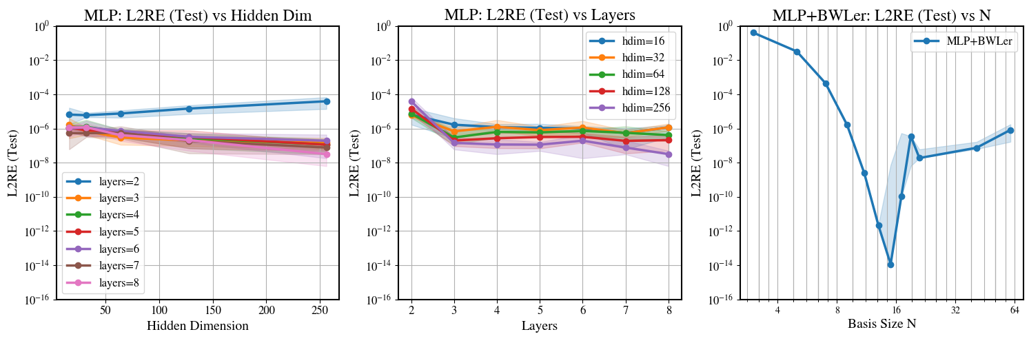
Multi-layer perceptrons (MLPs) plateau around relative error on 1D interpolation. BWLer-hatted MLP improves relative error by .
🎳 BWLer: Barycentric Weight Layer
Given polynomials perform so well on interpolation, why not directly incorporate them into a physics-informed model? That's exactly what our BWLer architecture is! Essentially, BWLer implements a spectral method into the auto-differentiable, physics-informed framework for PDEs, using polynomial interpolation as the core building block. BWLer supports two modes:
- In a BWLer-hatted MLP, BWLer acts like an extra layer atop a standard neural network.
- In explicit BWLer, BWLer replaces the neural network entirely and becomes an alternative architecture to MLPs.
This architecture shift yields dramatic improvements. We'll discuss the results in more detail in Part 2, but as a sneak peek, across three standard PDE benchmarks:
- BWLer-hatted MLPs reduce RMSE by up to .
- Explicit BWLer reaches up to RMSE — almost better than standard MLPs.
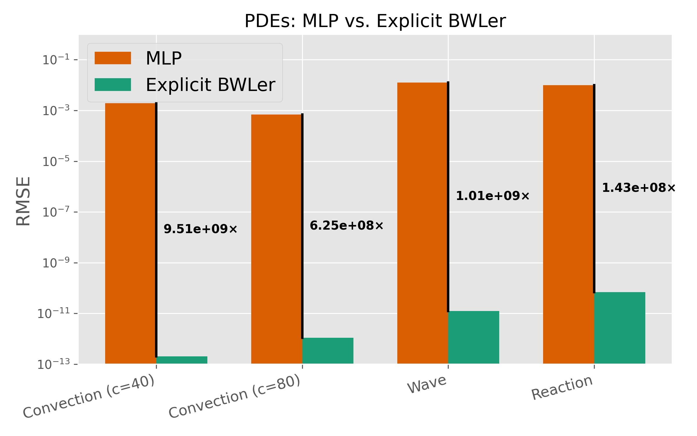
Sneak peek: on PDEs, BWLer outperforms standard MLPs — by up to 10 billion times relative MSE!
⏭️ What’s next in Part 2
So far, we’ve looked at the motivation behind BWLer, and seen that even basic function approximation is a challenge for standard PINNs. In Part 2 of this post, we’ll dive deeper into the technical details:
- How BWLer actually works under the hood
- What makes it more precise than traditional MLPs
- How it exposes and helps navigate a precision-conditioning tradeoff
We think there’s a lot more to explore here: from building better ML architectures for modeling PDEs, to designing systems that achieve higher precision, to maybe even moving beyond PDEs to fundamentally new tools for scientific modeling. BWLer is just a first step, and we’re excited to see what others might build from these ideas! Whether you’re trying BWLer out, adapting it to new problems, or just thinking about similar questions, we'd love to hear from you — please reach out and let us know what you're thinking about!
🛠️ Code & Resources
⏭️ Part 2 of the blog post
📄 Paper
💻 GitHub
📧 Questions? Reach out to jwl50@stanford.edu