Jun 8, 2023 · 26 min read
The Safari of Deep Signal Processing: Hyena and Beyond
Michael Poli, Stefano Massaroli, Simran Arora, Dan Fu, Stefano Ermon, Chris Ré.
New Models for Ultra-Long Sequences

Hyena takes a LLaMa to the safari.
The quest for architectures supporting extremely long sequences continues! There have been some exciting developments on long sequence models and alternatives to Transformers. Anthropic released an API for a model supporting 100k context length and Magic announced a model with 5 million context length (notably not a Transformer!). On the open-source front the RWKV team collected their insights into a paper and MosaicML got a Transformer to 65k context length with ALiBi positional encodings. We have also been hard at work - and would like to use this opportunity to share some of our research and perspectives on efficient architectures for long sequences based on signal processing.
We will start with a short definition of Hyena , then, through a historical note on efficient attention variants, we will attempt to outline a series of essential design principles for long sequence layers.
Part 1: What is Hyena?
The Hyena operator is a learnable nonlinear sequence processor. It can be utilized as a fundamental component in the construction of deep sequence models, such as for mixing information in the space (width) or time (sequence length) dimensions of the inputs.
The specific form of Hyena depends on its order. Here is the order case:
Hyena order-2 operator. (We use instead of for compatibility with the any-order case).
The core idea is to repeatedly apply fast linear operators (see 4.8 in Golub and Van Loan) -- operators that can be evaluated in subquadratic time -- to an input sequence , with every operator parametrized implicitly. In particular, the projections , which are mapped to the diagonals of , are produced by a fast linear operator on time and a dense linear operator over space. Often, we let be a Toeplitz matrix corresponding to an implicitly parametrized convolution filter . This means that instead of learning the values of the convolution filter directly, we learn a map from a temporal positional encoding to the values. Such a map can belong to various families; neural fields (e.g. SIRENs), state-space models (e.g S4) and rational functions.
The general order case follows directly1:
In Hyena and its predecessor H3 we argue that the above is a sufficient building block for large-scale language and vision models that rival Transformers in quality, while reducing the computational complexity to 2 -- for example, the cost of evaluating if is Toeplitz.
After close to a few months from the initial release, we have made progress on dissecting these learning primitives into essential elements. Before diving deeper, let's take a step back. How did we get here?
Our Goal: Attention
Attention is the fundamental operation in the Transformer architecture, which has led to significant progress in machine learning in recent years. Attention has some great properties: it can losslessly propagate information between any two entries in the sequence, regardless of their distance (global memory) and has the ability to extract information from any single element (precision). It is in some sense the best of both worlds, having perfect memory and perfect precision. However, it simply doesn't scale to ultra-long sequences, due to its quadratic computational complexity .
Dense Attention
The family of self-attention methods3 can be defined as
With , we obtain standard self-attention. Indeed,
Linear Attention for Linear Scaling
Many efficient alternatives to address the quadratic scaling of attention have been proposed -- we refer to this excellent survey.
One family of methods employs a simple low-rank factorization trick to achieve linear time scaling. The core idea can be summarized as:
That's it!4
Dissecting Linear Attention
We can dissect a linear attention layer into three steps: reduction, normalization and gating:
At its core, linear attention applies simple transformations to the input sequence: a (normalized) weighted combination, followed by elementwise gating. It uses two projections of the input, and , to parametrize the two operations.
While these approaches partially address the global memory property, they do so via a constrained parametrization (). Moreover, linear attention struggles at extracting information with precision (e.g. composing an output with a single input, far back in the past).
The AFT Variant
For example, the Attention-Free Transformer (AFT) flavor of linear attention proposes , yielding:
where is an elementwise nonlinear activation function. Note how the softmax is independent of the output index , yielding total linear time complexity.
The authors of AFT observed that with additional tweaks to they could further improve the results; in particular, they propose introducing more parameters to the exponential functions: . This new term represents one of the first instances of a method introducing additional trainable parameters (beyond the projections) in the linear attention decomposition. The choice of exponentials is natural given our starting point; with the linear attention factorization trick, these layers resemble simple state-space models.
Despite the changes, AFT still lags dense attention in quality. What can we do next?
RWKV for Precision
The RWKV team noticed that AFT and similar linear attention approaches cannot match quadratic attention on language modeling at scale. They proposed improvements to both the projections as well as the parametrization for . Let denote additional trainable parameters. Then, an RWKV (time mixing) layer5 is
RWKV makes the following key changes to AFT:
- Incorporation of previous element information in the projections , and .
- Restructuring of the parametrization towards exponential decay (intuitively: it appears to be a good idea to forget the past at some rate, and we have an extensive literature on recurrent networks that supports this).
With the new parametrization, the mixing operation can be shown to be equivalent to a linear state-space model (SSMs) with a single state (for each channel!). The convolutional form of RWKV is readily obtained as
where we have highlighted the role of as a pre-convolution gate.
Projections are often overlooked
But wait! The new projection is an extremely short convolution with filter size, with the elements of filters , and produced from a single parameter as and :
These modified projections allow the model to perform local comparisons and implement induction heads.
Building New Layers from Simple Design Principles
We have broken down linear attention-like approaches into four key components: projections, reduction, normalization, and gating. We are now ready to link back to Hyena! Let us discuss the elements that define Hyena and more broadly "safari" models.
Sifting for local changes
A key missing piece from previous efficient attention variants was a method to detect local (high-frequency) changes in the sequence. This is what the simple modification in the RWKV projections addressed, and can be generalized in various ways. Interestingly, a similar idea was proposed in the influential work on in-context learning via induction heads (the "smeared key" variant) as a way to enable even one-layer transformers to form induction heads.
In Hyena, we took the first step in generalizing the sifting operators in each projection, with short convolutional filters which excel at filtering the input to extract local features, as they can e.g. implement finite-differences to estimate derivatives, compute local averages and local differences. It can be verified that without the modified projections, any attention-free long sequence model performs worse on any task requiring in-context learning.
Memory over long sequences
The second core element is the reduction operator taking a history of values and aggregating them into an output. Luckily, there is no need to reinvent the wheel, tweaking the specific parametrization (the choices of in linear attention variants)! We can leverage an entire line of research on layers for long sequences, starting with seminal work on deep state-space models and follow-ups, that study exactly this question. Notably, these methods generalize and improve the expressivity of previous approaches using as reduction parameters. If the parametrization can be written in recurrent form, then the entire model can generate sequences at a constant memory cost, sidestepping the need to cache intermediate results.
Of course, there are trade-offs involved in different parametrizations, and in our experience these concern the scaling in quality over sequence length. In recent work, we attempt to quantify how much memory each reduction operator encodes, by measuring the minimum state dimension of the recurrence which approximates the convolution filter.
We found that for example, the implicit Hyena parametrization leads to larger recurrences than the H3 parametrization leveraging diagonal state spaces, providing some insight into our scaling results.
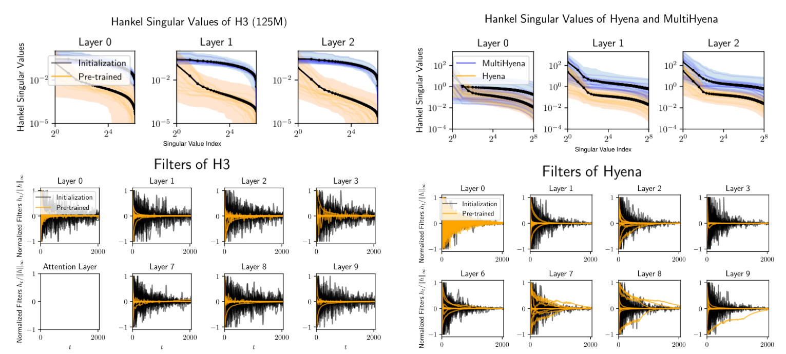
Spectrum of long convolution filters of Safari models (H3 and Hyena), alongside visualization at initialization and after pretraining. The decay rate depends on the reduction operator parametrization, with faster decays indicating correspondence to an equivalent recurrence with smaller state.
This is exciting because (a) it enables compression of long convolution layers into compact recurrences (smaller memory footprint, higher throughput, coming soon!) and (b) it provides a quantitative path towards further improving the parametrization for memory over ultra-long sequences.
We're also happy to highlight some recent results from our S5 friends: they replaced the existing implicit parametrization of long convolutions in Hyena with an expressive variant of state-space models, and achieved promising results. This is a very active area of research, and we fully expect to see improvements to the memory module that will further improve attention-free models!
Architectural considerations
So far, we have discussed the internals of the case. More choices open up as we consider a full Hyena block and operations that surround it
- Instead of having each operator act independently on each channel (space), we can form heads inspired by multi-head attention.
- A Transformer block is defined as attention followed by a small MLP. Turns out we do not need MLPs in Hyena models, provided we account for lost layers and floating point operations (FLOPs) when removing them. One option is to e.g. replace each MLP with another Hyena mixer, or introduce more FLOPs via heads.
Training efficiency
In addition to understanding the core machine learning ideas behind Hyena, it is important to characterize its efficiency, when mapped to modern hardware. Despite the improved scaling, Fast Fourier Transform (FFT) operations are poorly supported on modern hardware compared to operations such as matrix multiplication, which have dedicated circuits (i.e. NVidia Tensor Cores). This creates a gap between theoretical speedup and actual runtime. If the fast reduction operator of choice is a convolution, we have different options: (a) opt for parallel scans (e.g. the S5 approach) or (b) improve efficiency of the FFT. In some of our recent work, we address some of these challenges by using a single primitive — a class of structured matrices, called Monarch matrices, building on recent work from our lab. We develop a novel class of causal operators based on Monarch matrices that generalizes long convolutions and can be used as a drop-in replacement. Monarch matrices can be computed efficiently on modern hardware, using general matrix multiplications.
Monarch projections?
Another key question is how the parameter reduction incurred by swapping dense for sparse structured matrics in the projections -- beyond reductions -- affects model quality. This is exciting, because it leads us towards fully subquadratic architectures, in both width and sequence length. Here we provide some preliminary results and guidance for future work to extend Hyena.
We consider the associative recall synthetic task, in which sequences consist of key-value pairs (think of a dictionary). The keys and values are all single-character numbers and letters, and in each sequence the mapping varies. The model is tasked with providing the value for a key, given the sequence.
Intuitively, increasing the vocabulary size , i.e. the number of unique keys and values, is correlated with increased task difficulty. Note that in the above example, . Below, we vary , with and without replacing the Hyena projections with sub-quadratic structured matrices, and measure the validation accuracy.
| Vocabulary | Dense (2.2M params) | Sparse Structured ( 1.8M params) |
|---|---|---|
| 10 | 100 | 100 |
| 50 | 100 | 80 |
| 100 | 20 | 10 |
We observe the gap in quality between dense and sparse projections increases with task difficulty and are excited for future work to investigate this!
Inference efficiency
Inference workloads are incredibly important, especially when it comes to large language models. In fact, a lot of effort from the open-source community has gone into optimizing generation workloads so that they require less memory, can produce outputs faster, and can run on smaller devices. We study these questions in recent work that looks at distilling Hyena operators and other long convolutions into a recurrent form, using ideas from rational function approximation and model order reduction.
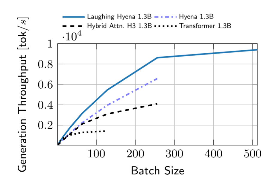
Throughput over batch size. Hyenas laugh when you distill them into a fast recurrence!
We are also able to take existing state-space approaches -- which already have a recurrent form -- and use our methods to prune redundant state dimensions, increasing throughput and reducing memory cost.
What's next?
This is only a snapshot of what we've been doing. We keep scaling in model sizes and sequence length. In other recent work, we pretrain Hyenas on up to million sequence length on genomics (at a "character" level), outperforming Transformers and efficient Transformers on downstream tasks, with much smaller models. Beyond these efforts, we are exploring various alternative parametrizations, much longer sequences, and looking further into character-level training. We continue exploring questions related to hardware efficiency and new applications of longer context lengths.
As always, we are most excited about finding deeper connections between our methods and classical signal processing and structured linear algebra.
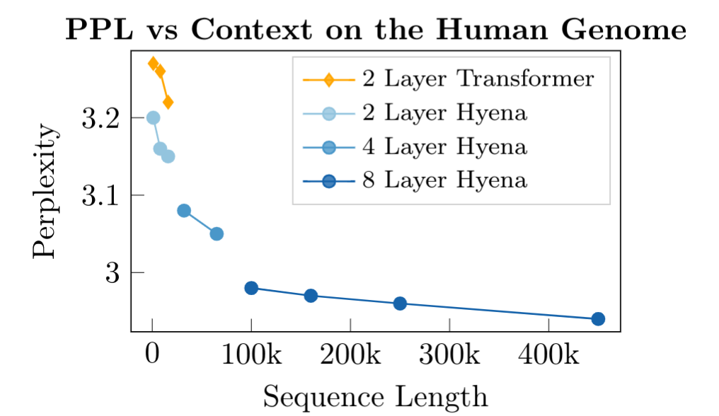
Pretraining on very long DNA sequences. Towards new scaling laws over sequence length.
Appendix: Hyena as (weak) time variance
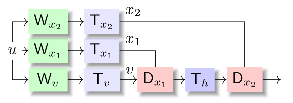
Consider a simple one-dimensional, discrete, weakly time varying6
The closed-form solution (input-to-output) reads (see this post or the classical book "Linear System Theory and Design" for a step-by-step reference in the time-invariant case):
What happened? If you look at the above, you might see something familiar: we ended up with the gate, long convolution, gate decomposition from order-2 Hyena operators. The main differences are of course due to the parametrization of each module in this input-output map. By using implicit parametrizations (for projections, and for the long convolutions) Hyena generalizes the above7 system.
With longer recurrences -- more gates and long convolutions -- we are in essence using chains of these systems. And there is something fundamental about operators that can be decomposed as chains of diagonal and circulant matrices.
Acknowledgments
Thanks to all the readers who provided feedback on this post and release: Avanika Narayan, Hermann Kumbong, Michael Zhang, Sabri Eyuboglu, Eric Nguyen, Krista Opsahl-Ong, David W. Romero.
- Note the change of notation from , to a generic for projections, as we have more than 3.↩
- Of course, it is a lot trickier to evaluate computational efficiency beyond asymptotics and floating point operations (FLOPs) - we will address this in an upcoming paper.↩
- Structural differences between different *sequence mixing layers (attention, H3, Hyena...) are more easily discussed in the regime, where denotes model width. Then each element in the input sequences is a scalar. The extension to the general case typically involves only a few choices -- keeping the dimensions independent, or aggregating into heads.↩
- In the scalar case, the simplify out. In the general vector case there is another small difference between AFT simple and general linear attention (see Sec 3.2).↩
- To clarify the connection between methods, we use the same notation for the projections. Forgive us RWKV team!↩
- This is not standard terminology, we use the term to indicate a system defined via (a) a time-invariant state-to-state transition and (b) time-varying input-to-state and state-to-output coefficients.↩
- We can characterize the result as an infinite-dimensional system, but that is beyond the scope of this post.↩