Jan 14, 2022 · 10 min read
Structured State Spaces: A Brief Survey of Related Models
Albert Gu, Karan Goel, Khaled Saab, and Chris Ré
In our first post, we introduced the motivating setting of continuous time series and the challenges that sequence models must overcome to address them. This post gives a (non-exhaustive) survey of some of the main modeling paradigms for addressing continuous time series -- recurrence, convolutions, and differential equations -- and discuss their strengths, weaknesses, and relationships to each other. In the next post, we'll see how state space models such as S4 combine the advantages of all of these models.
Three Paradigms for Time Series
How can we address these continuous time series? a few categories of end-to-end models have emerged, each of which addresses some of the above challenges while having other weaknesses.
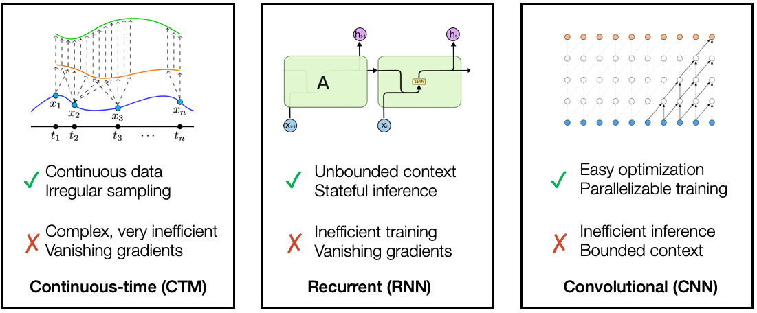
Strengths and weaknesses of common methods of modeling time series.
Recurrence: Beyond fixed windows
Recurrent models are perhaps the most classic and intuitive solution for sequential data. They simply store a representation of the context as a “hidden state” which is updated on a new input : . In deep learning, the update function is parameterized and these models are known as recurrent neural networks (RNNs). These models have been incredibly well studied over the years, with the most popular variants being the LSTM and GRU.
✓ Natural inductive bias for sequential data, and in principle have unbounded context
✓ Efficient inference (constant-time state updates)
✗ Slow to train (lack of parallelizability)
✗ In deep learning, long computation graphs cause the vanishing/exploding gradient problem
Convolutions: Easy to train
Roughly speaking, convolutional neural networks (CNNs) view an input sequence globally and pass through several rounds of aggregating data in local windows. Although CNNs are usually associated with 2-dimensional data, their 1-dimensional version is simple and can be a strong baseline for time series data. Their structure makes for simple features and obvious parallelizability. More sophisticated variants have shown strong results for certain types of long sequence tasks such as audio generation (e.g. WaveNet).
✓ Local, interpretable features
✓ Efficient training (parallelizable)
✗ Slow in online or autoregressive settings (has to recompute over entire input for every new datapoint)
✗ Fixed context size
Continuous-time: Exploiting the underlying structure
Very recently, a new paradigm for sequence models has emerged that treats a model’s activations or parameters as implicitly continuous. The most famous of these are neural ODEs which was introduced as a continuous-depth model, but have been generalized to continuous-time as an alternative to RNNs. Among other features, such models seamlessly handle continuous data such as addressing irregularly-sampled data in a principled way or automatic evaluation on data sampled at a different rate. Instead of standard backpropagation, models are trained with black-box ODE solvers and the adjoint method, which can be extremely slow.
✓ Automatically handles continuous data, e.g. irregularly-sampled data or test-time sampling shift
✓ Mathematically tractable to analyze, e.g. calculating exact trajectories or constructing systems for memorization (HiPPO)
✗ Extremely slow at both training and inference
Recent Progress in Combining the Paradigms
To address the downsides of existing models, recent work has found connections between these main paradigms that can combine their strengths. These models can acquire the efficiency and modeling benefits of multiple underlying paradigms.
Recurrent and Continuous-time
The connection from RNNs to continuous-time models have been known since their inception, and recent years have seen an explosion of CT-RNN (continuous-time RNN) models based on dynamical systems or ODEs. We briefly mention a few classic and modern works along these lines, categorizing them into a few main topics (note that some of these works may fall into multiple categories):
- Analysis of RNNs from a continuous-time point of view
- The correspondence between RNNs and dynamical systems has been studied (Niu et al. 2019) since the ‘90s (e.g. Funahashi & Nakamura 1993), with modern treatments focusing on analyzing the stability (Zhang et al. 2014) and dynamics (Jordan et al. 2021) of RNNs.
- RNNs designed to combat vanishing gradients using a dynamical systems analysis
- Several modern RNNs such as the AntisymmetricRNN (Chang et al. 2019), iRNN (Kag et al. 2020), and Lipschitz RNN (Erichson et al. 2021) address the exploding/vanishing gradient problem by reparameterizing the architecture or recurrent matrix based on insights from an underlying dynamical system.
- RNNs based on discretizing an underlying ODE from continuous-time to discrete-time
- coRNN and follow-up UnICORNN discretize a second-order ODE inspired by oscillatory systems.
- LMU and HiPPO-RNN – which are direct predecessors of S4 – use fixed, mathematically-derived linear dynamical systems
- LTC (https://arxiv.org/abs/2006.04439), CfC (https://arxiv.org/abs/2106.13898) : represent dynamical systems with varying time-constants with stable behavior and provable rates of expressivity measured by trajectory length
- Adapting a continuous-time model (neural ODE with adjoint method) to handle discrete inputs
- ODE-RNN, GRU-ODE-Bayes, ODE-LSTM extend adjoint-based neural ODEs to the discrete input setting as an alternative to standard RNNs
- NCDE, NRDE memory efficient versions that integrate observations more smoothly and can be extended to very long time series
Convolutional and Continuous-time
The connections between convolutional and CT models has been much less explored. The only example we are aware of is the CKConv (and followup FlexConv). Rather than storing a finite sequence of weights for a convolution kernel, the CKConv parameterizes it as an implicit function from which allows sampling it at any resolution.
To be precise, this method combines convolutions with implicit neural models (the best known examples of these is NERF) rather than with differential equations. This bestows it with certain properties of continuous-time models such as adapting to different resolutions, but doesn’t quite get other benefits such as having unbounded context.
Recurrent and Convolutional
Finally, there is a very simple connection between convolutions and a restricted class of recurrent models. Notice that a linear recurrence can be explicitly expanded out
in the form of a convolution
where is the convolution operator .
This observation was leveraged in the LMU-FFT to allow computing the LMU (mentioned above) much faster with parallelization, using the convolution theorem.
Why hasn’t this been used more? There seem to be two fundamental issues First, in terms of expressivity, this representation seems limited since it only applies to linear recurrences, whereas the most popular and effective RNN methods involve nonlinear recurrences. Second, in terms of computation, this actually doesn’t provide any speedup if the convolution filter has to be calculated, since that essentially involves unrolling the recurrence. The reason the LMU-FFT avoids this problem is that their matrix W is completely fixed (i.e. non-trainable), so that the convolution filter can be computed once and cached.
The Challenges of Memory (or Long-Range Dependencies)

A depiction of a typical ML sequence model.
At the beginning of this post, we laid out three challenges: efficiency, continuity, and memory. So far we’ve discussed the three paradigms and their abilities to address the first two challenges. Finally, we discuss the main issues for all models in addressing memory and recent progress.
RNNs, CT models: Vanishing Gradients, Speed
The main characteristic of RNNs - unrolling a function at every time step - means they are a natural model for sequential data that can in principle handle unbounded context. In practice, this is never the case, because these long computation graphs cause two significant problems. First, this directly causes the previously mentioned training efficiency issues. Second, chaining computations together can cause activations and gradients to grow exponentially in the length of the sequence, which is known as the “exploding/vanishing gradient problem”.
As previously mentioned, RNNs and ODEs are closely related, and CT models based on ODEs suffer from similar problems.
Addressing long-term dependencies has been the primary problem for RNN models to overcome. However, it still remains a substantial challenge: very few methods seem capable of handling sequences significantly longer than 1000 to a few thousand steps, outside of synthetic tasks. Instead of listing a small subset of the innumerable works on this subject, we highlight a few of the only methods known to us that have been evaluated on sequences of length at least 10000.
- The LMU and HiPPO derive a closed-form ODE which provably memorizes the history of a function in continuous-time, and show that these can remember toy tasks for 100000 or longer steps. However, converting these into a trainable RNN adds components that reintroduce the main drawbacks of RNNs
- The UnICORNN discretizes a coupled system of second-order differential equations that has gradient bounds and an efficient CUDA implementation, allowing it to scale to long sequences
- Neural Rough Differential Equations (NRDE) compress the input signal on small time intervals using the log-signature method, improving the speed and memory of neural ODE-RNN methods
Convolutions: Fixed Windows
In practice, convolutions can be used to cover long distances when combined with tricks such as pooling or dilated convolutions. However, they are still fundamentally a fixed window model that can’t hope to handle unbounded context. As data scales up and we move to more complex applications with longer and longer sequences in areas such as speech and video, and start to tackle “life-long” or continual learning, these models (and other fixed-window models such as transformers) are fundamentally limited.
Summary
In this post, we discussed the three major classes of models used to address time series, recent progress in combining some of their strengths, and their fundamental difficulties with long sequences. In the next post, we discuss our new model which combines the strengths of all three paradigms discussed here to address the challenges of continuous time series.