Jan 14, 2022 · 22 min read
Structured State Spaces: Combining Continuous-Time, Recurrent, and Convolutional Models
Albert Gu, Karan Goel, Khaled Saab, and Chris Ré
In our previous post, we introduced the challenges of continuous time series and overviewed the three main deep learning paradigms for addressing them: recurrence, convolutions, and continuous-time models. We discussed their strengths and weaknesses, and summarized recent progress on connecting these families of models.
In this post, we show that the connections between these paradigms run deeper, and in fact there is a very simple and fundamental continuous-time system that underlies recurrent and convolutional models.
The State Space Model (SSM)
The continuous state space model (SSM) is a fundamental representation defined by two simple equations:
Here the input is a 1-dimensional signal, the state is a N-dimensional latent representation satisfying a linear ODE, and the output is a simple 1-dimensional projection of the state. Here is called the state matrix, and the other parameter shapes are .
The state space model is a fundamental representation used in many scientific and engineering disciplines such as control theory, statistics, and computational neuroscience, and is also related to latent state models such as Hidden Markov Models and Kalman filters. Conventionally in these areas, the system parameters are assumed to be latent (i.e. fixed) and the goal is to either control the system (find inputs that lead to desirable outputs ) or use a noise model to perform statistical inference on quantities such as the parameters or state.
In our work, we simply use the state space as a black box representation in the spirit of deep learning, where we view an SSM as a function-to-function map parameterized by parameters which are simply learned by gradient descent. In order to do this, let’s concretely see how to compute this layer.
Three Representations of SSMs
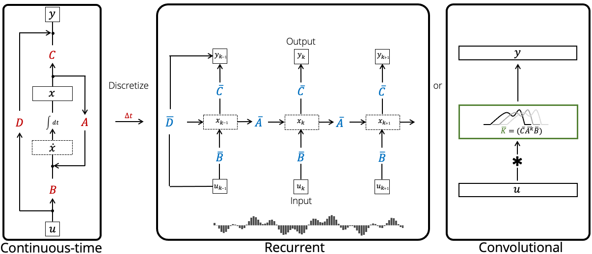
A key feature of the SSM is that it has three different representations, which allows it to be viewed (and computed) as a continuous-time, recurrent, or convolutional model. Furthermore, these representations can be "swapped" for each other to get different properties depending on what's most useful for the application. This is extremely useful because we saw in the previous post that these three paradigms offer distinct computational and modeling advantages.
The Continuous-time Representation
The main representation of the SSM is the one given above. We denote the parameters of this continuous-time representation in red:
In control theory, the SSM is often drawn with a control diagram where the state follows a continuous feedback loop.
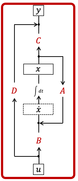
We think of this as a function-to-function map parameterized by . Note that this representation is mostly theoretically; we won't be receiving data in the form of closed-form functions so we can't directly apply this representation. However, this is the base form from which the others will be computed, and offers the most intuition into the model's behavior.
Computing the SSM with Recurrence
Real data is discrete, so what we want from a sequence model is to be able to transform an input 1-D discrete sequence (instead of a continuous input signal ) with a parameterized map. Mechanically, the linear ODE can be simply turned into a linear recurrence that maps to an output sequence , one step at a time:
Here the parameters of the recurrent model are , which have simple closed formulas in terms of the base parameters .
There are actually many formulas that are valid, but the one we use in S4 is called the bilinear transformation which is given by
Note that this involves choosing a fifth parameter which represents a step size or the granularity of the input data. We'll defer the discussion of these formulas for now.
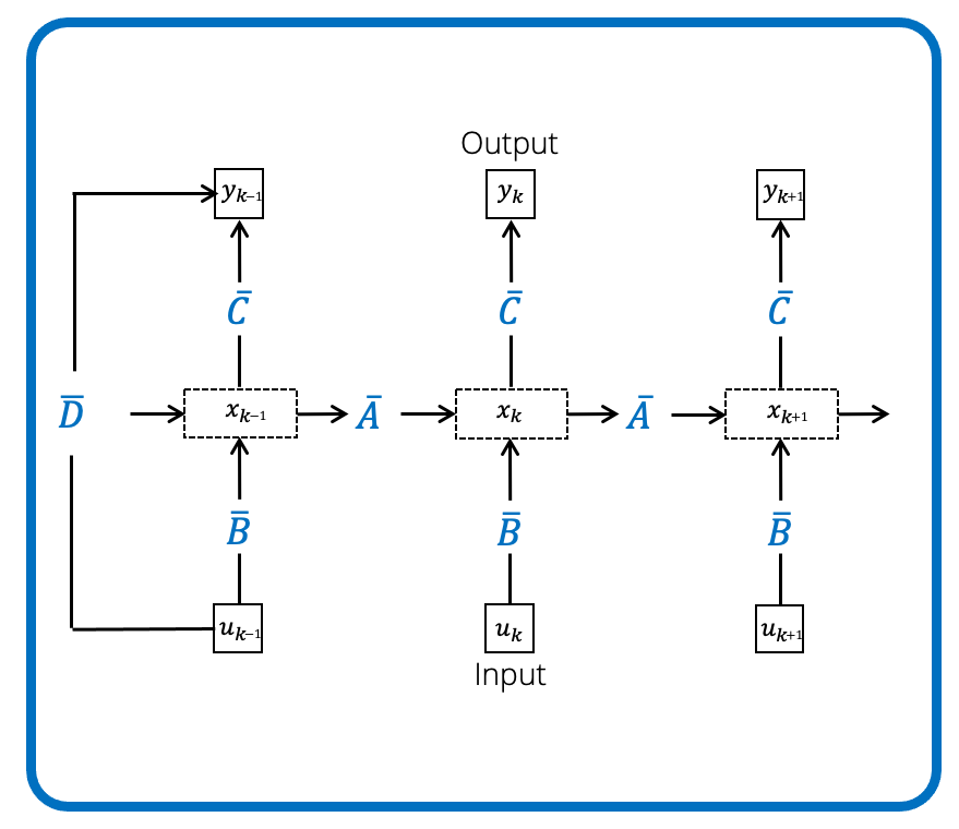
Computationally, this looks just like a simple RNN where the inputs are processed one at a time, getting combined into a recurrent hidden state , and linearly projected to an output .
Computing the State Space with Convolutions
As mentioned in the previous post, it's been observed that linear recurrences can be computed in parallel as a convolution! To see this, the above recurrence can be explicitly computed to reveal a closed formula for the output in terms of the input . First, the state is unrolled by repeated multiplication.
Then the output is a simple linear projection of the state.
We end up with a simple closed form for the outputs at every step :
By extracting these coefficients into what we call the SSM kernel
this means that the entire output of the SSM is simply the (non-circular) convolution [link] of the input with the convolution filter
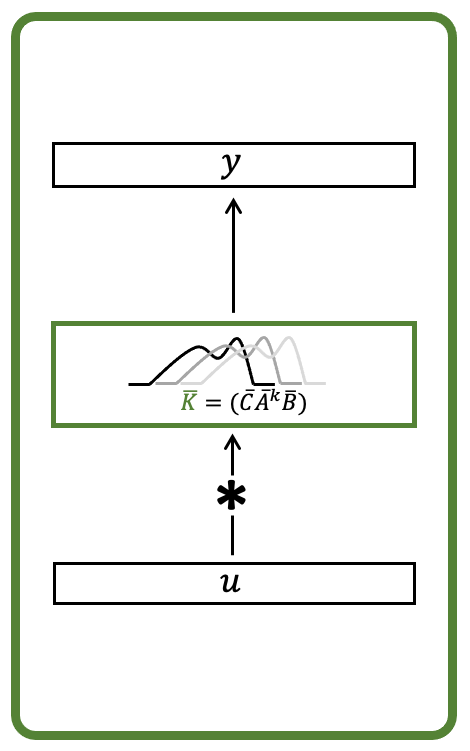
This representation is exactly equivalent to the recurrent one, but instead of processing the inputs sequentially, the entire output vector can be computed in parallel as a single convolution with the input vector .
What does it mean to be continuous-time? A discussion on discretization
While the convolutional representation of SSMs is straightforward to derive from the recurrent representation with just a few lines of math, with a simple expression for the convolutional parameter in terms of the recurrent ones, we've skipped over the details of how the recurrent representation was derived. What are the formulas for in terms of ? In what sense are the continuous-time and discrete-time models equivalent?
This is one of the biggest departures from traditional sequence models, and we offer a few different views and intuitions to interpret it.
Interpretation 1: Interpolate and apply continuous-time model
Convert discrete-time sequence into continuous-time signal, then apply continuous model
Perhaps the simplest way conceptually to think of the discrete-time (sequence-to-sequence) model is to first convert the input to continuous-time, then apply the original (function-to-function) model. This process is illustrated below.
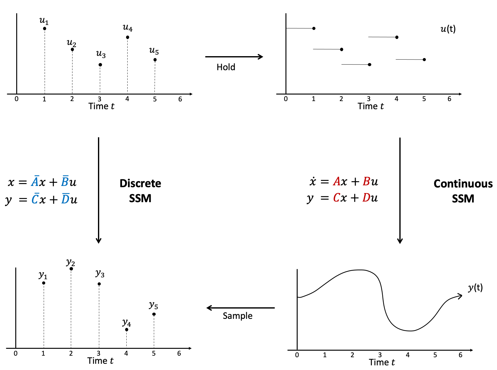
The discrete-time SSM (left), a sequence-to-sequence map, is exactly equivalent to applying the continuous-time SSM (right), a function-to-function map, on the held signal.
This simple "interpolation" (just turn the input sequence into a step function) is called a hold in signals, as it involves holding the value of the previous sample until the next one arrives. Its advantage is that with a simple linear model such as the SSM, the original continuous model can be exactly computed yielding a closed form.
In order to do this, we require a step size to hold each sample for - S4 also treats this as a learnable parameter.
Then the discrete SSM with formula
is exactly equivalent to the continuous SSM on the held signal. The Wikipedia page on discretization has a nice derivation.
Finally, some other discretization methods can be seen as approximations of this formula; for example, Euler's method uses the approximation while the bilinear transformation that we use is the first order Pade approximant .
Interpretation 2: Recurrent approximation with numerical integration
A second way to derive the discrete-time models is through numerical simulation of the dynamical system. More broadly, these techniques write a differential equation in integral form and then approximate the integral with numerical integration techniques.
To illustrate, the simplest method approximates the integral with its left endpoint, . This is known as Euler's method which simulates the differential equation with a simple linearization .
Applied to (the first equation of) the SSM, we get
where we have defined . This would be one valid set of discretized SSM parameters from Euler's method.
Other methods of approximating the integral yield different formulas. Using the Trapezoid rule gives a more accurate approximation, which leads to the bilinear transformation formula that we use in S4.
Interpretation 3: Changing the width of the convolution kernel
What happens if we drop all the other representations for now and view the SSM simply as a discrete convolution? Then decreasing can be seen as "stretching out" or "smoothening" the kernel.
Why we want to do this should make sense intuitively. Suppose we're operating on input data sampled at an extremely high rate, so that samples from one time to the next don't change too much. Then it wouldn't make sense to have a very spiky convolution kernel where each element is completely independent of its neighbors - we want the kernel to be smooth like the signal.
Another way of seeing this mechanically is that as , the discretized state matrix becomes closer to the identity , so the kernel becomes smoother!
What about other integration methods?
There's a rich literature of numerical methods for differential equations, which offer different tradeoffs in approximation accuracy.
For our purposes, we have a couple of desiderata for our discreted SSM:
- Accurate: It should approximate the underlying continuous model accurately
- Time-invariant: We want the discretized SSM to involve a recurrence that looks the same at every step, allowing it to be unrolled into a convolution. Furthermore, we can't choose the points where we observe function values; these are given to us and we assume they're uniformly spaced
- Causal: We can't look ahead to see samples in the future, which is required by some integration methods
- Efficient: It should be fast to compute the recurrence parameters and to step the recurrence
These requirements led us to the bilinear transform used in S4. In HiPPO, we also experimented with the zero-order hold (ZOH) used in HiPPO's predecessor and found that its performance was comparable to the bilinear transform, so we've stuck to the bilinear transform since then for its simplicity and theoretical efficiency. (The main difference is that the bilinear method involves only matrix multiplications and inverses by , which can be done in linear time when is a structured matrix as in S4, whereas ZOH requires a matrix exponential which takes cubic time.) We're unsure whether more sophisticated discretization methods might also be viable, which may be an interesting question to look into for the future!
Comparing the SSM representations
To summarize, here's a quick diagram recapping the different representations of SSMs and how they're related to each other.
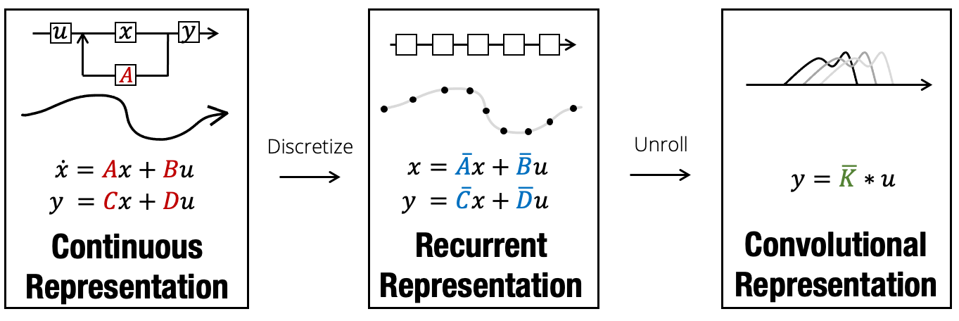
Swapping between these representations is powerful: the state space layer acquires the benefits of all types of models outlined in the previous post, including:
- adapting to new sampling rates (continuous-time representation)
- unbounded context, efficient autoregressive generation (recurrent representation)
- fast, parallelizable training (convolutional representation)
In this section we'd like to discuss further some of the consequences of these representations, as well as how SSMs compare to more traditional models.
The Continuous-time SSM
What's the advantage of having a continuous-time model?
First, one benefit is that it's easier to analyze continuous models. This was a main theme of the HiPPO paper which started the S4 line of work: working with functions instead of sequences allowed for a new mathematical framework for "continuous-time memorization", which could be analytically solved into new tools for processing signals.
Second, CTMs seem to have better inductive bias for modeling "continuous data". Empirically, S4 showed the strongest results on the types of continuous time series defined in the first post in this series, such as audio signals, sensor data (e.g. ECG measurements), image data from raw pixels, and weather and energy time series. On the other hand, some types of data such as text isn't continuous in the same sense - it was not sampled from an underlying physical process - and correspondingly we found that S4 didn't perform as well.
Finally, a concrete advantage of CTMs is that they can handle tricky settings such as irregularly sampled time series, missing data, and changes in sampling rates. On the speech classification experiment in the S4 paper, we took the S4 model trained on 16000Hz data and tested it on 8000Hz waveforms. Doing this requires simply doubling the value of at test time! Our discussion about discretization above should make it intuitively clear why this works.
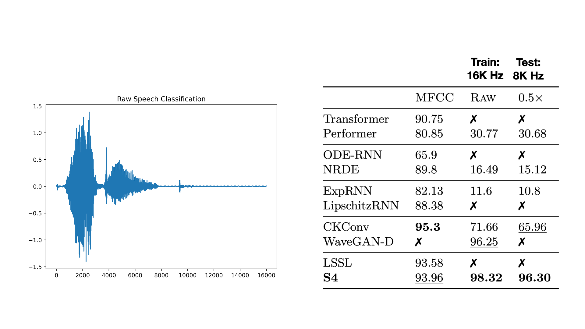
A trained S4 model can adapt to any sampling rate at test time by simply changing its step size !
Here are a few common questions that we've gotten about this capability:
- Although we only showed what happens with downsampling the signal, it would also work with upsampling
- We chose a factor of 2 because of convenience; it's the simplest way to create data with a different sampling rate. However, we're aware that this leads to some trivial baselines (e.g. to go from 8000Hz to 16000Hz, just downsample at test time; to go from 16000Hz to 8000Hz, just duplicate every sample at test time).
- We emphasize that this experiment would work for any change in sampling frequency. We suspect that results should be more accurate the closer the shift is to .
RNNs vs SSMs
One of the main strengths of RNNs is the ability to model data statefully - an RNN keeps track of all the information it's seen into a context. As a modeling advantage, this makes them naturally suited for settings that are naturally sequential and stateful, such as modeling agents in POMDPs. As a computational advantage, this means that processing a new step always takes constant time, instead of scaling with the size of the context (as in Transformers and CNNs).
As an example application, we showed that a trained S4 model (using the convolutional representation) could be switched into the recurrent representation to drastically speed up autoregressive generation.
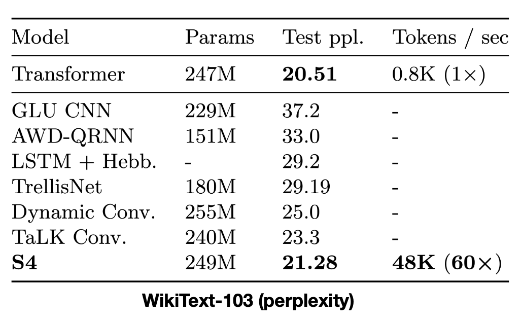
S4 sets SotA for attention-free models, while generating tokens 60X faster than a parameter-matched Transformer by switching to its recurrent representation at generation time.
SSMs also have a few disadvantages compared to RNNs.
How can an SSM model nonlinear dynamics?
A key feature of the SSM is that it's a linear model, which drastically simplifies its computation and allows it to be computed fast (by unrolling into the convolutional representation). However, this seems like it might be less express compared to nonlinear RNNs.
- In the LSSL paper, we show theoretically that a "single layer" non-linear model can be converted (at least locally) into a deep model where each layer has linear dynamics and with pointwise non-linear transformations between layers.
- We note that some of the more recent RNNs such as the Quasi-RNN and Simple Recurrent Unit use architectures that have simple (essentially linear) recurrences similar to the SSM, allowing them to be much faster than more complicated RNNs while performing better.
- We also note that CNNs are similar to SSMs in that they are composed of linear layers (convolutions) with non-linear transformations in between.
Empirically, we have found S4 to be better than all RNN baselines (such as the LSTM) in every application we've tried. Of course, we've mostly investigated difficult long-range modeling tasks where RNNs have known shortcomings, but the results seem quite promising.
What about variable sampling rates?
So far we've assumed that the step size is constant, but there may be settings where we want to model non-uniform rates. By using an SSM in recurrent mode, it is possible to capture this by discretizing with a different at every step (this can be given in the data, or chosen by the model in an input-dependent way, etc.). Note that this feature is common to many other types of CTMs as well and RNNs based on continuous dynamics surveyed in the previous post.
However, we note that by doing this, the convolutional equivalence is lost. So in practice we have never tried this with S4, as the convolutional representation is very important to be able to train on long sequences.
CNNs vs SSMs
The connection between convolutions and state spaces is actually much more straightforward and follows from classic results in signal processing. In short, taking the Laplace transform of the SSM shows that , where is called the impulse response of the system and is a rational function of degree . Conversely, it is well known that convolution by any rational function of degree can be expressed as a state space representation. So in the limit as the state size tends to infinity, the state space can represent any convolution!
When training an SSM in convolution mode, it resembles a standard CNN quite closely. A main difference is that instead of local convolutions, the SSM convolution kernel is infinitely long - this is a convolution in the traditional signals sense. This means that as opposed to CNNs, which require carefully designing neural network architectures that involve hierarchical receptive fields and pooling or dilations, SSMs can be simply stacked with repeated blocks like Transformers.
In practice, we found that while S4 generally performs as well as comparable CNNs while requiring much fewer parameters, it can be slower to train. Part of this might just be engineering - our implementation of these global convolutions involves several rounds of FFTs that should be optimizable into a fused kernel.
To Be Continued...
This post discussed the various representations and tradeoffs of state space models compared to CTMs, RNNs, and CNNs. However, SSMs have notable drawbacks that have previously prevented them from being used in deep learning. For example, although we've elaborated on the advantages of having multiple representations, it turns out that actually computing these representations is extremely slow - a consequence of the fact that the SSM has a much higher state dimension than its input/output dimension. In future posts, we'll talk more about how S4 overcomes these problems and how S4 was developed. For now, we recommend checking out details in the original paper, as well as the excellent Annotated S4 post.