Dec 11, 2023 · 24 min read
Zoology (Blogpost 2): Simple, Input-Dependent, and Sub-Quadratic Sequence Mixers
Based: An Educational and Effective Sequence Mixer

We’re excited to share our new ~ Based ~ architecture, inspired by our theoretical and empirical analysis of how different architecture classes perform associative recall (AR), a key task predictive of language modeling and in-context learning capabilities.
Key takeaways: Based is a simple architecture that combines two familiar sub-quadratic operators: short convolutions and linear attention. These operators have complementary strengths and together enable high-quality language modeling with strong associative recall capabilities. At inference time, because Based only uses fixed-sized convolutions and linear attentions (computable as recurrences), we can decode with no KV-cache. This enables a 4.5x throughput improvement over Transformers with Flash Attention 2.
We demonstrate these properties along three axes, finding that Based provides:
- Simple and intuitive understandings: we motivate
Basedwith the view that simple convolutions and attentions are good at modeling different kinds of sequences. Instead of introducing new complexities to overcome their individual weaknesses, we can combine familiar versions of each (short 1D convolutions! “spiky” linear attentions!) in intuitive ways to get a best-of-both-worlds situation. (Section 1. Introducing theBasedModels)
- High quality modeling: despite its simplicity, in our evaluations we find
Basedoutperforms full Llama-2 style Transformers (rotary embeddings, SwiGLU MLPs, etc.) and modern state-space models (Mamba, Hyena) in language modeling perplexity at multiple scales. (Section 2.Basedoutperforms Transformers in language model perplexity.)
- Efficient high-throughput inference: when implemented in pure PyTorch,
Basedachieves 4.5x higher inference throughput than competitive Transformers, e.g., a parameter-matched Mistral with its sliding window attention and FlashAttention 2. High throughput is critical for enabling batch processing tasks with LLMs. (Section 3.Basedis fast.)
This blogpost is the first preview of Based, lots more to come! You can follow along with our downstream language modeling results in this WandB report and play with Based on our synthetic associative recall testbed in this repository.
Section 0. Recapping the lessons we learned in Zoology.
In our previous blogpost, Zoology: Measuring and Improving Recall in Efficient Language Models, we discuss the analysis that motivated the design of Based. Here’s a quick summary of what we learned…
We found that there is a small perplexity gap between recently proposed sub-quadratic gated-convolution architectures and Transformers, when training on fixed data (10B tokens of the Pile) and infrastructure (EleutherAI GPT-NeoX). However, after performing a fine-grained error analysis, we see there remains a significant gap on next-token predictions that require the model to deploy a skill called associative recall (AR).
What’s AR? Consider the sequence: “She put vanilla extract in her strawberry smoothie … then she drank her strawberry ?” – the model needs to be able to look back at the prior context and recall that the next word should be “smoothie”. We find that the gated-convolution models’ poor performance on these sorts of token predictions account for >82% of the remaining quality gap to attention on average! A 70M attention model outperforms 1.4Bn Hyena on AR tokens.
| Attention | Long Conv | Hyena | H3 | RWKV | |
| All Tokens (PPL) | 9.44 | 13.13 | 10.38 | 10.07 | 9.79 |
| AR Tokens (PPL) | 1.98 | 13.27 | 4.81 | 3.83 | 3.82 |
| Other Tokens (PPL) | 10.62 | 13.12 | 11 | 10.75 | 10.51 |
Table 1: Perplexity of 355 million parameter models trained for 10 billion tokens on the Pile.
Yet, some subquadratic gated-convolutions match attention on the non AR slice! Can we capture the strengths of both gated convolutions and attention in one purely sub-quadratic architecture?
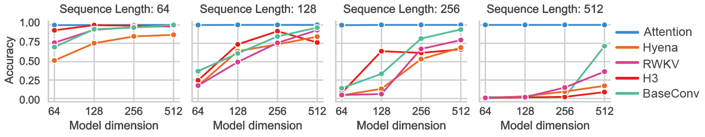
We find the AR gap is because gated convolution models (e.g. Hyena, H3, RWKV, RetNet) need model dimension that scales in sequence length to solve associative recall. We can see this scaling on synthetic associative recall data:
Is there a path forward without quadratic attention? Finally, we saw with theory and experiments that we need input-dependent sequence aggregation in our architecture to solve the proposed multi-query associative recall (MQAR) as efficiently as attention. Again, attention computes Softmax(QKT), where Q and K are functions of the input data u, to determine how to mix tokens. Convolutions use a fixed filter, defined by the model weights, across diverse inputs.
Section 1. Introducing the Based Models
We now introduce Based, a new approach to subquadratic sequence modeling. Motivated by the findings above, we set out to test a simple hypothesis: convolutions and attentions seem naturally complementary; if we combine their capabilities, can we get a simple architecture that outperforms both?
To do so, we build Based around two key primitives: (1) short gated-convolutions and (2) spiky linear attentions. Intuitively, the standard convolutions in (1) are great for modeling local dependencies and settings where we might not expect to need associative recall (think building up morphemes [i.e., units of meaning] from individual tokens, similar to how in vision we build up higher-level features from neighboring pixels). Meanwhile, the linear attentions in (2) enable Based to do associative recall, e.g., by recovering the global “look-up” inductive bias of standard attention 1.
As we’ll see, the combination of both enables Based to achieve high quality sequence modeling while remaining *fully sub-quadratic*. Aside from its aesthetic appeal, we’ll further see that keeping everything sub-quadratic unlocks other niceties of Based, such as its high-throughput generation capabilities via no KV cache.
Finally, for those of you that insist on architectural purity, you’ll be pleased to find that we can also unify the modules of Based as two sides of the same architectural block. Under this view, each layer of Based can be viewed as a gated convolution, depending on how we parameterize the filter weights.
In the remainder of this post, we’ll first go over the gated convolutions and linear attentions of Based under their intuitive interpretations for local sequence modeling and global look-ups / associative recall. We’ll then provide a short overview of the unified view of Based. We’ll finally present our Based evaluations, discussing its high-quality language modeling and high-throughput generation capabilities.
Building Block 1: A Simple Short Gated Convolution
To build Based models, we start with short convolutions, as we like their subquadratic efficiency and their ability to model local interactions. As a review, these standard short convolutions have fixed-length filters directly defined by model weights. By “sliding” these filters over an input sequence, we thus only scale linearly in sequence length. Furthermore, because these filter values *are* neural net weights, by training the layers we directly learn the local relations between neighboring tokens as neural net parameters.
Inspired by recent works and our own results showing improved performance with gating (especially on non-AR slices where some gated convolutions even outperformed attention), we further make these layers gated. Under first principles, this allows us to better model settings where neighboring token interactions are still somewhat context-specific; the “gate” modulates the weights based on its input token.
# No gating, relation defined by fixed k1, k2, k3 for all x
y3 = k1 * x3 + k2 * x2 + k1 * x1

# Gating, relation dynamically modulated by x3
g3 = g * x3
y3 = (g3 * k1) * x3 + (g3 * k2) * x2 + (g3 * k1) * x1
However, unlike these works, we leave the long-range modeling to the linear attention layers we describe next. In this way, we let convolutions do what they do best, and avoid the complexities of trying to get them to scale to longer sequences 2.
In our experiments, we use two sets of filters of length 3 and 128. This lets us capture both higher and lower frequency features within local contexts (i.e., token patterns that repeat a lot versus those that occur more sparsely).
v = conv1D(u)          // filter size 3 ("short")
v = F.SiLU(v)
v = conv1D(v)          // filter size 128
w = Linear(u)          // projection on dimension
w = F.SiLU(w)
y = v * w              // gating
Building Block 2: A Spiky Linear Attention
Next, we need a simple way to solve AR (and MQAR) sub-quadratically. We already know that attention is great at this; the softmax between queries and keys enables a kind of “look-up” perfect for doing this context-based recall that we’re after.

However, even the latest-and-greatest versions of attention like FlashAttention2 are quadratic in time over sequence length (and further won’t enable our high-throughput generation discussed later on).
So how do we enable this attention-like behavior while remaining subquadratic? We revisit the great ideas in *linear attention*. On our visit though, we add in a simple twist inspired by recovering this “look-up” capability that seems so important for associative recall (at this point it’s really just haunting us).
Linear attention - all you need?
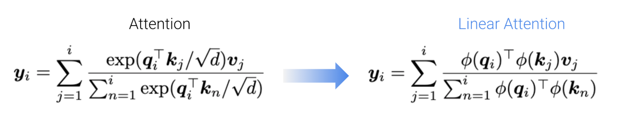
We start by reviewing a really cool idea from Katharopoulos et al. 2020. In this seminal linear attention paper, the authors note that if we take standard attention, but remove the softmax around our query-dot products, the resulting outputs can be computed in linear time!
Just computing these scaled query-key dot products alone doesn’t seem to work, so folks usually further transform the queries and keys with element-wise “feature maps” . The key challenge is picking which feature maps to use.
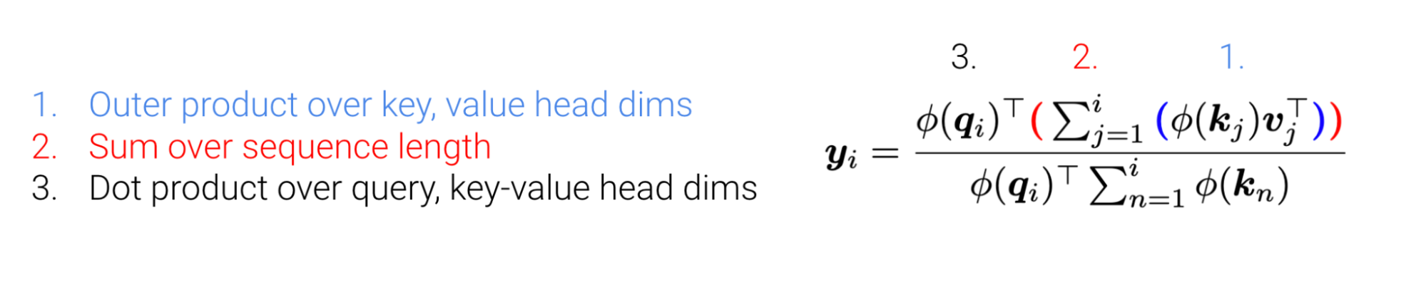
Digging into the efficiency a bit, by rearranging which matrix multiplications we compute first, we can compute attention in O(ndd’) time and space for sequences of length n, if queries and keys are size d’, and values are size d.
Now this is great, because typically head dimensions are much smaller than the sequence length. However, there does lie a rub.
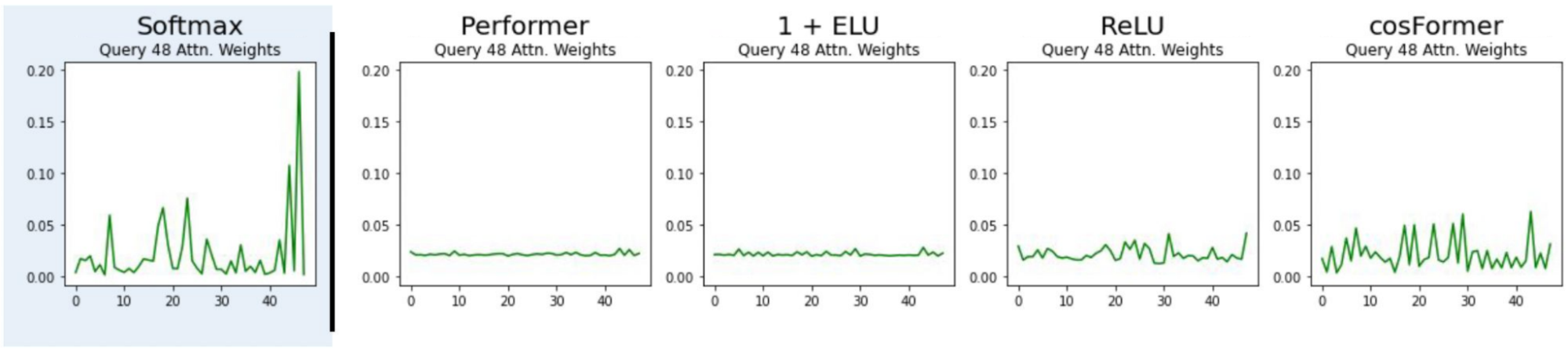
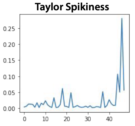
Unfortunately, when we tried existing feature maps, we found they too struggled to learn associative recall. This was perhaps surprising, given the theoretical guarantees of past inspiring methods designed to approximate the exponential function in standard attention (e.g., random fourier features from Rahimi & Recht, 2007, Choromanski et al., 2020). Inspecting the actual linear attention maps or weights, we found that in practice, without scaling up head dimension the actual attention weights produced were much more uniform (higher entropy) than softmax, i.e., “less spiky”. Intuitively, this is bad because this prevents us from paying “attention” to tokens of interest versus, exactly what we want attention to do for AR!
| Softmax | 1 + ELU | ReLU | Performer | cosFormer | Taylor Exp (Based) | |
| Acc (%) | 100.0 (0.00) | 17.07 (0.58) | 10.88 (1.32) | 15.14 (1.27) | 15.82 (0.48) | 100.0 (0.00) |
Table 2. Associative Recall (AR) task performance for different linear attentions. Mean accuracy % (and stdevs) over 5 seeds. Previewing a bit, we make a Based linear attention that solves AR just like standard softmax attention!
The Taylor Exponential - high-school calculus is all you need
In the midst of trying to get these prior methods to work better, we came across a surprisingly simple solution: approximating the exponential with a Taylor series. In short, by computing such that , we were able to compute attentions with similar spikiness to standard softmax, at head dimensions small enough to remain relatively efficient.
In slightly more detail, the linear attention algorithm above is a bit like a “reverse” kernel trick. Instead of trying to come up with a function such that (saving us from computing a higher-dimensional dot product; over the head dimensions), we want to come up with a function such that computing (saving us from computing a large outer product; over the sequence length).
Exactly computing with ’s requires infinite-dimensional features; no good. But with just the second-order Taylor series, where , we can make this tractable! Our feature maps simply exploit the linearity of the dot products, where we first compute the feature maps for each Taylor series order before summing their dot products.
In pseudocode:
# Compute zero-order terms
qk0 = 1  # 1

# Compute first-order terms
q   = [q1, ..., qd]
k   = [q1, ..., qd]
qk1 = (q * k).sum()  # qk

# Compute second-order terms
q = [q1 * q1, ..., q1 * qd, ..., qd * q1, ... qd * qd]  # flattened qq^T
k = [k1 * k1, ..., k1 * kd, ..., kd * k1, ... kd * kd]  # flattened kk^T
qk2 = 0.5 * (q * k).sum()  # (qk)^2 / 2

# 2nd-order Taylor exp: 1 + qk + (qk)^2 / 2
y = qk0 + qk1 + qk2
As above, if queries and keys are originally size , then the resulting dot products take time and compute. The overall linear attention then takes time and space. In practice, we simply choose a smaller head dimension for queries and keys to make this trade off favorable for more sequences. As shown below, we find this retains better-than-Transformer modeling quality with d = 16 and d = 24 in the model results below, making us 16x and 4x faster than naïve attention for seq len = 4096, (128x and 32x faster at seq len 32k if we’re counting).
All your Based are gated convolutions
While the hybrid view of Based above conveys its modeling quality, for the architectural purists we can also interpret the short convolutions and linear attentions as two instantiations of the same (generalized) gated convolution block.
Note that a convolution takes in two input signals and u (the "kernel" and "input") and produces an output signal y, denoted as . The unified Based parameterizes overall kernel K via learnable short filter queries , and keys , and parameterizes inputs as values , where , , and are all linear projections of layer inputs .
Where for , let and .
For our first short convolution block. We set the first K filter values as learnable weights, setting the rest of the signal to 's: We "ignore" all queries and keys (setting them to ones or the equivalent constants for multiplicative identities), and set the value projection to the identity matrix, computing inputs u as the layer's inputs (model's hidden states).
For our second linear attention block. For basic linear attention, we set the filter f to be the ones vector n:
It's a bit weird at first, but this just highlights that vanilla linear attention does not permit position-dependent modeling. To add this in, as a nice connection to relative positional embeddings such as ALiBi, we can also cover these cases and include positional dependence by instantiating the filter as positional embeddings, e.g., to dictate some exponential decay. We then learn the query, key, and value projections.
In this sense, linear attention is also a gated convolution. The dot products of pairwise queries and keys, each a projection of the original layer inputs, act as an input-dependent "long convolution" filter (stretching all the way back to the beginning of the sequence, e.g. when computing attention weights ). After multiplying with f (optionally enabling relative positional encoding), these then "gate" or interact with the layer's inputs via the values (the layer inputs transformed by the value projections, ala and ).
Recap
There is a plethora of new sub-quadratic models, so we pause to reflect on some of the considerations that researchers and users might pay attention to, when deciding where to start. We focus on simplicity and exposition in our design.
-
Simplicity. The operations (1D convolutions, projection, and gating) are very familiar to ML practitioners from PyTorch 101 and the layers require no specialized initialization scheme or filter biases, as compared to recent architectures like Hyena and Mamba. The model is stable to train in BF16 precision with low/no effort.
-
Interpretability. The block is also simple to theoretically analyze (see our paper for more on this), since all operations are polynomial operations. In our paper, we provably analyze our gated convolution layer showing it provably simulates all gated convolution architectures (H3, Hyena, RWKV, RetNet, etc.).
-
Efficiency. We also note that in contrast to prior work (H3, Hyena, Striped Hyena, Multi-Head Hyena, M2, BIGS, etc.), the block does not use convolutions where the filter is as long as the input sequence. The use of short convolutions plus linear attention permits parallel training and recurrent inference, without requiring any further modifications like distillation.
Section 2. Based outperforms Transformers in language model perplexity.
In this section, we’ll present some of our initial experiments with Based! These empirical results answer the following questions:
-
Can
Basedreplicate the associative recall capabilities of attention? -
Can
Basedmatch attention in overall language model perplexity?
Synthetic Associative Recall Testbed
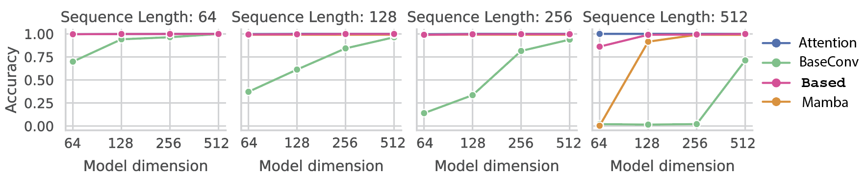
In our previous blog post, we discussed why, relative to attention, gated-convolutions (e.g. BaseConv, Hyena, RWKV) struggle to perform associative recall. We used a synthetic associative recall task to demonstrate that gated-convolutions require the hidden state to scale linearly with the sequence length (see BaseConv in the plot below). In contrast, we show that Based (and the recently proposed Mamba architecture) both are able to solve associative recall at (almost) all sequence lengths with constant model dimension.
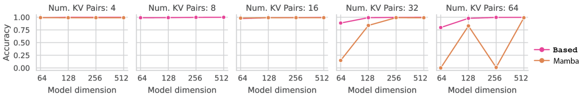
We also stress test Based (and Mamba) on a harder version of associative recall with more and more key-value pairs. Intuitively, it is difficult to “store” all the keys and values in a single RNN hidden state. Intuitively, both architectures fall off in performance as we increase the number of KV pairs.
So, at least on synthetics, Based largely replicates the associative recall capabilities of attention. What about real language?
Language Modeling Quality on the Pile
We train Based on the Pile language modeling corpus at 150m and 350m parameter scales, finding that Based outperforms the very strong Llama Transformer baseline (with rotary embeddings, GLU, etc.) by a sizable margin. Critically, with Based, we close 98% of the gap to Attention on the challenging associative recall slice.
Expand below for a detailed description of the experimental protocol.
Experimental protocol: We train each model for 10B tokens on the Pile (same exact data and data ordering) using the EleutherAI GPT-NeoX training infrastructure. The data was tokenized using the GPT2BPETokenizer. We report the overall test perplexity at the end of training as well as results for the AR and non-AR slices of next-token predictions.
We train all models using the same Llama-style architectural backbone (i.e. SwiGLU MLPs, Rotary embeddings when applicable), simply swapping the sequence mixer. However, for Mamba, RWKV, and RetNet, we also change the broader block as these architectures use specialized state mixers. For each model, we take the best training configurations we can find from published papers, GitHubs, and HuggingFace. Note that tables of training configurations are included in our Zoology paper along with the citation for the sources of hyperparameters.
We also keep the following hyperparameters constant across training runs: learning rate and learning rate schedule (warmup 1% of iterations with a max LR of 8e-4), optimization (Adam), global batch size (500K tokens), normalization (pre-norm for the sequence mixer and MLP), precision (BF16, using FlashAttention V2 for high-precision attention, residuals in FP32, etc.), weight decay (0.1), and gradient clipping (1.0).
At the 150M parameter scale.
| Model | Parameters (M) | Overall PPL | AR PPL | Non-AR PPL | % of gap explained by AR |
| Transformer++ | 125 | 11.01 (2.40) | 2.16 (0.77) | 12.45 (2.52) | - |
| H3 | 168 | 12.06 (2.49) | 6.75 (1.91) | 12.60 (2.53) | 88.4% |
| Hyena | 158 | 11.60 (2.45) | 5.00 (1.61) | 12.28 (2.51) | 100% |
| RWKV | 169 | 11.64 (2.45) | 5.70 (1.74) | 12.29 (2.51) | 100% |
| RetNet with window size 128 attention | 152 | 11.15 (2.41) | 3.01 (1.10) | 12.45 (2.51) | 100% |
| Based Feature dim 16 | 163 | 10.34 (2.34) | 2.37 (0.86) | 11.56 (2.45) | - |
At the 350M parameter scale.
| Model | Parameters (M) | Overall PPL | AR PPL | Non-AR PPL | % of gap explained by AR |
| Transformer++ | 360 | 9.44 (2.25) | 1.98 (0.69) | 10.62 (2.36) | - |
| H3 | 357 | 10.38 (2.34) | 4.81 (1.57) | 11.00 (2.40) | 65.8% |
| Hyena | 358 | 10.07 (2.31) | 3.83 (1.34) | 10.75 (2.38) | 98.2% |
| RWKV | 351 | 9.79 (2.28) | 3.82 (1.34) | 10.51 (2.35) | 100% |
| Mamba | 358 | 8.99 (2.20) | 2.07 (0.73) | 10.15 (2.32) | - |
| Based Feature dim 16 | 360 | 9.08 (2.21) | 2.08 (0.73) | 10.15 (2.32) | - |
| Based Feature dim 24 | 362 | 8.88 (2.18) | 2.02 (0.70) | 9.93 (2.30) | - |
Table 3: Test perplexity (PPL, cross-entropy loss in parentheses) of sequence models trained for 10 billion tokens on the Pile.
Section 3. Based is fast. Fast is based.
Based enables dramatic improvements in throughput.
Language model throughput, the number of generations an LLM can complete per second, is the salient performance metric in a majority of industry applications of LLMs. For example, when an LLM provider (e.g. OpenAI or Anthropic) is serving requests behind an API, a model’s throughput determines how many queries can be served from a fixed set of GPUs. Moreover, much of our economy depends on batch processing systems that run at scale behind the scenes, including systems for everything from processing financial transactions to managing supply chains to analyzing scientific and health data. For these tasks, it’s throughput that matters, not latency.
LLMs could revolutionize these batch processing tasks, but their throughput lags behind more efficient alternatives (e.g. fine-tuned BERT). The throughput of existing attention-based LLMs is bottlenecked by the KV-cache, which grows in the length of the generation and limits the possible batch size. Eliminating the KV-cache is a key motivation for the design of Based. Because linear attention can be viewed as a recurrence and short convolutions only require computing over the last filter-size terms during generation, Based’s hidden states only require constant memory; no KV-cache or growing with generated sequence length!
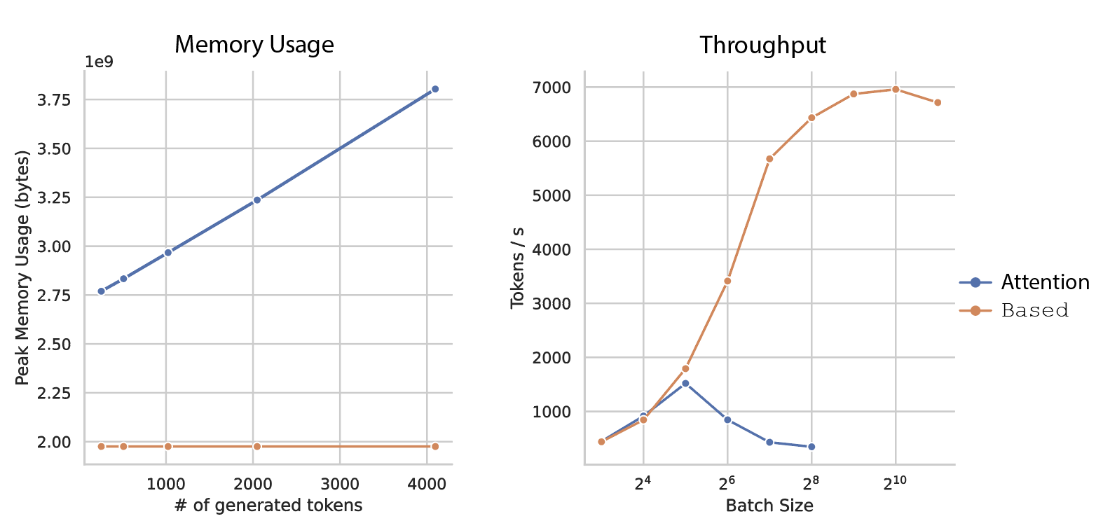
We benchmark on a single GPU a 1Bn parameter Based model against a 1Bn parameter Mistral Sliding-Window Attention model. In the plot below and to the left, we see that the peak memory usage of Attention grows linearly with the number of generated tokens in order to store the KV-cache. In contrast, it stays constant when using Based because the KV state is of fixed size. This difference in memory consumption makes a huge difference as we increase the batch size. At low batch sizes (< 32), Attention and Based are indistinguishable. But as the batch size increases, the KV-cache in attention grows so large that the overhead of managing the memory hurts throughput and, eventually, it just runs out of memory. At its peak, Based can generate 6,959 tokens per second. In contrast, the best average throughput for Attention is 1,519 tokens per second. This represents a 4.58x improvement in throughput.
Training Speed.
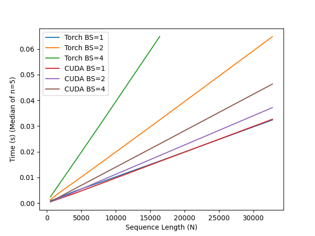
Finally, we implement an IO aware algorithm for computing the linear attention QKV interactions. First recall the reads and writes that could hurt the efficiency of our linear attention layer in practice. Recall that our linear attention feature map for Q and K is a Taylor approximation of the exponential function applied to q and k respectively. Including the second-order term in the approximation results in an tensor, for sequence length and for feature dimension . We then perform a matrix multiplication between Q and KV , where is value head dimension. Writing and reading these matrices to and from slow HBM would inhibit the efficiency of Based.
We split the QKV computation into three blocks for the zero-order, first-order, and second-order Taylor approximation components. We load a tile (16 x 16, the size of a Tensor core) of q, k, and v per warp. Within each warp, we can compute the causal linear attention locally. We can then perform a global causal linear attention given the local results. Note the hidden dimension of q, k is simply feature dimension , where is often 16 (the dimension of the Tensor Core GEMM, funnily enough also what we find sufficient for good performance) – this allows us to perform the computation in this tiled fashion.
In early evaluations across sequence lengths for varied batch sizes (BS), we compare the PyTorch reference implementation provided here, with the CUDA code and observe the following speedups! Note that the PyTorch code runs out of memory at N=32768 and BS=4. Experiments are run on an 80GB A100 GPU.
Conclusion
With this post, we hope to illustrate how we can achieve high quality and throughput, all while sticking to familiar architectural building blocks. We’re continuing to scale up Based, sharing preliminary results in this WandB report. If interesting, definitely don't hesitate to reach out and please follow along! (We :heart: collaborators and compute :) )
We'd like to thank Dan Fu and Hermann Kumbong for providing valuable feedback on this blog post. Also a special thanks to Together for providing the compute to train our models!
- It’s worth pointing out that similar discussions and ideas have played out with our vision community friends. For example, Convolutional Vision Transformers (CvTs) (Wu et al., 2021) apply 2D convolutions to build local features, before patching and passing these to later attentions to model global relationships. ↩
- While remaining stable to train, parameter-efficient, and efficient-to-compute.↩