Efficient language models as arithmetic circuits

This blogpost was written as a resource in conjunction with our talk at STOC 2024. It focuses on work done with the following full team: Michael Zhang, Aman Timalsina, Michael Poli, Isys Johnson, Dylan Zinsley, Silas Alberti, James Zou, Christopher Ré.

---

The Transformer architecture, which powers most language models (LMs) in industry, requires compute and memory to grow quickly with the input size during training and inference, precluding dreams of modeling inputs containing millions of lines of code or the 3.2Bn nucleotide pairs in genome sequences. Alternative architectures (e.g. Mamba, RWKV), which seek to reduce the compute and memory requirements relative to Transformers, are emerging at a rapid pace. However, deviating from the Transformer orthodoxy is a major risk: models are served to millions of users and take billions of dollars to train, and we have limited insight into how switching to these alternatives might impact quality.

Thus, we need frameworks to reason about which architectural changes matter and why. We’ve been writing a series of papers that use arithmetic circuits to make some sense of the landscape of architectures (Zoology, Based, JRT). Our general approach is to view each architecture as different a arithmetic circuit, a composition of sums $(+)$ and products $(\times)$, and to reason about the efficiency of different LMs in terms of the number of operations required to perform tasks of interest. This post describes our theoretical results.

Part 1: A single skill, associative recall, causes a lot of trouble

It is difficult to reason about language modeling quality given the breadth of skills involved (e.g. fact memorization, in-context learning) and the many different levels of abstraction for skills (e.g. some work evaluates LM’s grammar skills while others evaluate an LM’s ability to “emotionally self regulate”). We decided to train a bunch of LMs across architectures and do error analysis to see what we’d find!¹

Error analysis across efficient LM architectures

Surprisingly, we found that a single skill called associative recall (AR) glaringly stood out in the error analysis: Transformers crushed it and the efficient LMs struggled. An LM performs AR if it recalls information that it has seen earlier in the input. For instance, LMs need to refer to functions or variables that already exist in the inputted codebase when generating subsequent lines of code. Our prior posts here and here dive more into our empirical observations. As a recap:

1. Gated convolutions. We found 80%+ of the language modeling quality difference between Transformers vs. the class of “gated convolution” LMs (built from gating and convolution operations e.g., H3, Hyena, RWKV) is attributed to AR. We find these LMs perform abysmally on in-context learning (ICL) tasks that require performing recall (e.g., document question answering, information extraction).

Next, training other classes of LM architectures, including selective state space LMs (e.g. Mamba, GateLoop) and linear attention LMs (e.g. GLA, Based), at 1.3Bn parameters, 50Bn tokens, and evaluating on ICL tasks that require performing recall (FDA, SWDE, NQ), we found:

2. Selective state space models. For 1k and 2k length documents, Mamba underperforms the Transformer by 42% and 55% on average across tasks.
3. Linear attention. There is excitment around linear attention since they extend the Pareto frontier of the efficiency-recall quality tradeoff space beyond the above architecture classes. Still, Based underperforms the Transformer by 27% and 41% at 1k and 2k length documents on average.

This blogpost focuses on how we theoretically explore what's going on with AR.

Formalizing the associative recall problem

Based on our analysis, we defined the MQAR problem: An LM needs to refer back to key-value token mappings (on the left) to answer questions (on the right). Here the answers are 4, 6, 1, 2.

$\textrm{A 4 B 3 C 6 F 1 E 2} \rightarrow \textrm{A ? C ? F ? E ?}$

Formally, given an input sequence $x = {x_0, . . . , x_{N−1}}$ where each $x_i \in C$ is a token drawn from a vocabulary of size $c = |C|$. The task is to check, for every query $1 \leq i < N$, whether there exists a $0 \leq j < i$ such that $x_i ≡ x_j$. If so, output $x_{j+1}$.²

Theoretically reasoning about open-ended problems like language modeling is complicated, but the simplified MQAR task helped us make some progress. When we train LMs on synthetic MQAR data (like the example above), the trends correlate with real language modeling gaps between architectures trained to large scale. Prior work has extensively explored AR over multiple decades (Graves et al., 2014, Ba et al., 2016, Schlag et al., 2021, etc.). We find MQAR quality correlates better with real language modeling quality than previously used formulations (discussed in more detail in our prior blogpost).

---

Part 2: Background

Here we'll briefly recap the definitions of different sequence mixers and intuition on why our efficient LMs might struggle to perform MQAR.

Sequence mixers are the part of an LM that determines how words in input $x \in \mathbb{R}^{N \times d}$ for sequence length $N$ and model dimension $d$, interact with each other when computing output representations $y \in \mathbb{R}^{N \times d}$ for the subsequent layer of a deep neural network.

First we'll start with the de-facto attention sequence mixer, and then describe two (closely related) categories of efficient LMs: linear attention and state space models. The LMs shown in Figure 1 above all fall in these two categories.

Attention models mix tokens as follows:

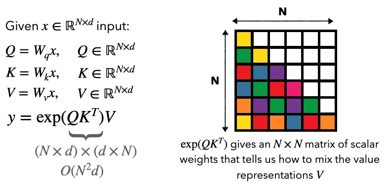
Attention takes $O(N^2d)$ compute and linear $O(Nd)$ memory during training. During inference, remember we generate one token at a time $t$ -- each new query $Q_t$ needs to interact with all the prior $K_{0:t}$ and $V_{0:t}$ so if we cache those keys and values, compute and memory to generate a token scales with $t$.

Linear attention models, proposed by Katharopoulos et al., 2020 replaces $\exp$ with a “feature map” $\phi: \mathbb{R}^{N \times d'} \rightarrow \mathbb{R}^{N \times D}$, with “feature dimension” $D$. As before, $d$ is the model dimension, but we’ll decouple $d’$ so $Q$ and $K$ can be projected to a different dimension than $V$ as needed.

Shown in the figure, this is now $O(NDd)$ linear in $N$ during training. During inference, by summing prior $h_t = \sum_{i=0}^{t} \phi(K_t^T) V_t$ such that $h_t \in \mathbb{R}^{1 \times Dd}$, then multiplying this with $Q_t$, observe our compute and memory to generate a token is constant $O(1)$ as $t$ grows.

State space models The mixing proceeds as follows:

And many SSM variants also use Hadamard product (elementwise multiplication between $2$ vectors) operations in addition to the convolution.

This ignores that SSMs are continuous objects, for a more precise definition see prior blogs. Observe that we again have a recurrent view ($O(1)$ compute and memory) we can use during inference and a sub-quadratic parallel convolution $O(dN \log N)$ with FFT view we can use during training.

Intuition on why gated convolutions may struggle on MQAR Before diving into the theory, let's make sure we have some high level intuition on why efficient LMs might struggle. MQAR requires us to compare tokens to find matching tokens, and then shift forwards the answer for the next token prediction.

Attention computes inner products between all tokens, making it easy to find matches! In the above figure, note the convolution is more restricted, a Toeplitz matrix, so a token can only be compared to a token $4$ positions prior if all tokens compare to the tokens $4$ positions prior to them as well. The comparisons are accomplished by using a convolution filter that shifts the sequence $4$ positions. Once we shift, the model can compare the shifted and original sequences to identify matches using the aforementioned Hadamard products.

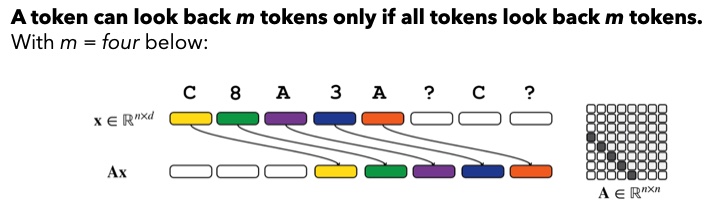
In our convolution models, we apply a unique convolution filter for each of the $d$ dimensions, so we can support multiple shifts. BUT, to support all $O(N)$ possible shifts in a sequence of length $N$, each hidden effectively needs to store information about all tokens to be able to perform the comparison.

Okay so we have some intuition on why convolutions might struggle -- the filters are input-independent and it's hard to support all the shifts with small model dimension. Attention's input-dependent mixing is helpful to find the matching tokens. We walk through this intuition more slowly in our prior blogpost.

---

Part 3: Unifying the messy architectural landscape using arithmetic circuits

Above, we walked through a toy construction of how LMs might solve MQAR, but there's a messy landscape of LMs with subtle modifications from architecture to architecture. We use theory to reason about the landscape systematically.

Towards this, we first observe our efficent LM classes (gated convolutions, linear attentions) can be written as polynomials in terms of the input variables! The models we consider are maps $M:\mathbb{R}^{N\times d}\to \mathbb{R}^{N\times d}$ and each of the $Nd$ output values are polynomials in the $Nd$ input variables $x[i,j]$ for $(i,j)\in [N]\times [d]$.

Polynomial view of the primitive operations in efficient language models

Gated convolutions. Let’s walk through how Hadamard product and convolution operations are expressed as polynomial operations. Suppose we have two vectors:

$x = [x_0, x_1, …, x_{N-1}]$

$v = [v_0, v_1, …, v_{N-1}]$

First, recall that a Hadamard product between vectors $x$ and $v$ computes: $y = [x_0 v_0, x_1 v_1, …, x_{N-1} v_{N-1}]$. Note that here the $N$ outputs $x_i\cdot v_i$ is a degree $2$ polynomial in the variables $x_i$ and $v_i$.

Next, a convolution between vectors $x$ and $v$ computes (for $0\le i\le 2N-2$):

$(x \ast v)[i] = \sum_{j=0}^{i} x_{i-j}v_j$.

We can see that each of the $2N-1$ outputs are polynomials in the $2N$ inputs variables in $x$ and $v$. In models that use convolutions typically $v$ is fixed (it is a learned convolution filter), so the convolution becomes a linear operator– i.e. for each of the output positions we compute a polynomial of degree at most $1$.

Linear attention models We can express each entry of the $(i, j) \in \mathbb{R}^{N \times d}$ linear attention output as a polynomial as follows. We let $D$ be the feature dimension and $Q, K \in \mathbb{R}^{N \times D}$ and $V \in \mathbb{R}^{d \times d}$ be our embedding projections.

$h_{i,j}(x) = \sum_{m \in [D], n \in [N]} (W_Qx)[i, m] \cdot (W_Kx)[n, m] \cdot (W_Vx)[n,j]$

We can see that this computes a degree $3$ polynomial at each position (three variables from input $x$ are being multiplied).

!! Note !! One limitation of the arithmetic circuit view is that we can’t exactly represent non-polynomial activation functions, like the $\exp$ in attention or Mamba. However, foreshaddowing a bit, we will use functional approximation theory to approximate $\exp$ with (small degree) Taylor polynomials for $\exp$.

Measuring the efficiency of models using arithmetic circuit complexity

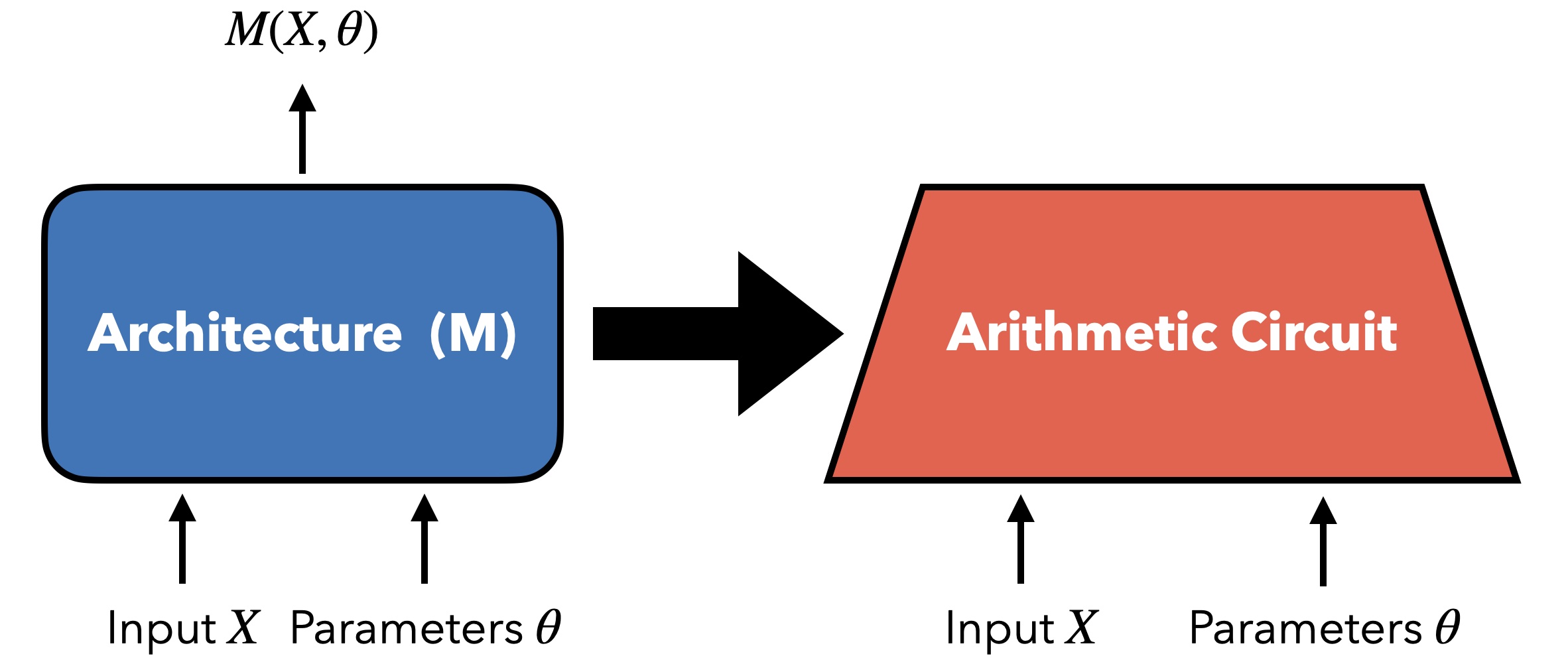
All gated convolution models (Dauphin et al., 2016, H3, BiGS, Hyena, RWKV, M2, etc.) and linear attention models (with polynomial feature maps) are polynomials, which means they can be directly computed by arithmetic circuits! Efficient ML is all about the scaling needed to obtain some desired quality, and there are many ways to define efficiency e.g., data, compute, parameters: here we use the complexity of arithmetic circuits as our measure of efficiency. Arithmetic circuits provide a natural and powerful computational model for studying the complexity of polynomials, with deep connections to fundamental problems in theoretical computer science. The complexity of a polynomial is determined by the size of the smallest arithmetic circuit that computes the polynomial.

What is an arithmetic circuit? An arithmetic circuit is a directed acyclic graph that represents a polynomial function of the circuit’s input variables. We can express our polynomial (gated convolution) as arithmetic circuits with our input $x$ and model parameters $\theta$ as inputs. Each node in the circuit is an addition ($+$) or multiplication ($\times$) operation between inputs.

As an example, let’s express the Discrete Fourier Transform (DFT) as a linear arithmetic circuit for an input $v$ of length $n=4$ (Dao et al., 2020). Linear means the circuit uses just linear gates (i.e. gates on input $x$ and $y$ compute $ax+by$ for constants $a$ and $b$), contrasting general arithmetic circuits, which also have multiplication gates (i.e. on input $x$ and $y$ compute $xy$).

An arithmetic circuit is an $(n, s, \Delta, \omega)$-circuit, if it takes $n$ variables, has size $s$, depth at most $\Delta$ and width $\omega$. The size is the number of nodes in the circuit, depth is the length of the longest path between input and output nodes, and width is the maximum number of wires that cross any “horizontal cut” in the circuit. If we implement a DFT by doing the naive $O(n^2)$ time algorithm, then for the order 4 DFT matrix, we have 4 rows (4 inner products). To implement each inner product we need 3 linear gates for an overall 12 linear gate ops. But here, we show the FFT algorithm, using fewer (8) linear gates.

Quick notes on arithmetic circuits, polynomials, and structured matrices

Feel free to skip this section if you're familiar with these concepts

Again, when we talk about arithmetic circuits being equivalent to polynomials, we are talking about outputting $Nd$ values $y[i,j]$ by computing polynomials with respect to the $Nd$ input variables (e.g., $x[i,j]$) in $x \in \mathbb{R}^{N \times d}$ . Each polynomial has a single output value, so the model/circuit computes $Nd$ polynomials, which as mentioned before, are each of degree at most $2$ in the case of convolutions plus Hadamard product, and degree $3$ for linear attention.

In our prior tutorial blogpost on polynomials and convolutions, we thought about polynomials in the coefficient space, whereas in all our discussion in this blogpost, our polynomials are in evaluation space. Why? Well, for the convolution case discussed in our prior blogpost, we were picking the evaluation points, namely we chose the complex roots of unity as our evaluation points permitting us go back and forth between coefficient and evaluation spaces (we could take the DFT of the coefficient vector in order to evaluate the convolution (polynomial)).

Why did we think about coefficients in the Monarch Mixer work? Well, we cared about causality, which is fundamentally about the positions of different tokens governing which other tokens they can interact with in the context -- so, we chose a polynomial basis to help us analyze that property.

Reminder of the polynomial basis considered in our prior work

Let’s also write $[x_0, x_1, …, x_{N-1}]$ as coefficients of a polynomial $f(Z)$ and $[v_0, v_1, …, v_{N-1}]$ coefficients of $g(Z)$:

$f(Z) = x_0 + x_1Z + …. + x_{N-1}Z^{N-1}$

$g(Z) = v_0 + v_1Z + … + v_{N-1}Z^{N-1}$

First, recall that a Hadamard product between vectors $x$ and $v$ computes:

$y = [x_0 v_0, x_1 v_1, …, x_{N-1} v_{N-1}]$

By definition, the Hadamard product of two polynomials is obtained by element-wise multiplying the coefficients of the polynomials. I.e.:

$f(Z) \odot g(Z) = x_0 k_0+x_1 k_1 Z+ \dots+ x_{N-1} k_{N-1} Z^{N-1}$

The $Z$ powers remain unaffected because they are part of the polynomial's structure (corresponding to the positions in the sequence), not the elements being operated on. The operation preserves the polynomial’s form, altering only the coefficients.

Second, a convolution between vectors $x$ and $v$ computes (for $0\le i\le 2N-2$):

$(x \ast v)[i] = \sum_{j=0}^{i} x_{i-j}v_j$

This is equivalent to multiplying the two polynomials whose coefficients are provided by $x$ and $v$ respectively: $h(Z) = f(Z)g(Z)$,

or

$h(Z) = ( x_0 + x_1Z + …. + x_{N-1}Z^{N-1} ) ( v_0 + v_1z + … + v_{N-1}Z^{N-1} )$,

Which is the same as

$h(Z) = \sum{i=0}^{2N - 2} w_i Z^i$.

In the above, each coefficient is:

$w_i = (x \ast v)[i] = \sum_{j=0}^{i} x_{i-j}v_{j}$.

Meanwhile, arithmetic circuits need to work for all potential evaluation points - we can't pick our evalution points. Taking in the $Nd$ input variables, arithmetic circuits can use arbitrary computations to compute the $Nd$ outputs (sharing computation across the $Nd$ polynomials within the circuit)!

Another way to think about things. We can move between coefficient and evaluation space in general: polynomial evaluation at $N$ points is equal to multiplying by a structured Vandermonde Matrix containing the polynomial coefficients! However, for Vandermonde matrices, the arithmetic circuit conversion has complexity $O(N \log^2 N)$ arithmetic operations -- this is a bad way to express the circuits since it's a large number of operations and could result in numerical stability issues. In general, Vandermonde matrices are ill-conditioned, but the DFT, a special case of Vandermonde matrices, has condition number $1$ (i.e. is very well conditioned).

Hopefully this helps you think about why we choose different polynomial bases across these works. Alright, let's get back to the main story!

Unifying efficient LM architectures via the polynomial view

This section unifies architectures using the polynomial view.

Gated convolutions. Using the polynomial view, we first prove that any gated convolution model (including H3, BiGS, Hyena, RWKV, M2, etc.) can be simulated by a single canonical representation, BaseConv, within tight (poly)logarithmic factors in model parameters and depth. Given an input $u \in \mathbb{R}^{N \times d}$, the BaseConv operator on the right is defined as:

where $h \in \mathbb{R}^{N \times d}$ contains learnable filters, $W \in \mathbb{R}^{d \times d}$ is a linear projection, and $b_1, b_2 \in \mathbb{R}^{N \times d}$ are bias terms. The $\odot$ represents a Hadamard product and the $\ast$ represents a convolution. Each BaseConv layer is a polynomial of degree at most $2$ since the left and right sides are linear (degree $1$) in input $u$, and taking their Hadamard product, two linear polynomials get multiplied together.

Linear attentions. We prove that an $(N, O(log2(Nd)), d, O(N(d + D)), O(\max(d, D)))$-BaseConv (using $(n, s, \Delta, \omega)$-circuit notation) computes the output for a single linear attention layer with feature dimension D. This points to the relative efficiency of linear attention over gated convolutions: we need multiple BaseConv layers to represent one linear attention layer.

Moreover, we can convert any arithmetic circuit into a BaseConv model with only a poly-log loss in parameters:

Theorem (Arithmetic circuit equivalency). For every low-depth arithmetic circuit of size $s$, depth $\Delta$, that takes $u \in \mathbb{R}^{N \times d}$ as input, there is an equivalent BaseConv operator that uses $\tilde{O}(s\Delta)$ parameters and $\tilde{O}(\Delta)$ layers.³

For specific instantiations of gated convolutions (e.g., Hyena models), we show in our paper that we can even get rid of the poly-log factor, where $\tilde{O}(\cdot)$ hides poly-logarithmic factors.

Why is this theorem exciting to us? Let's walk through a few implications of this theorem:

1. Arithmetic circuits are non-differentiable objects. However, BaseConv is differentiable, allowing us to reason about how things actually learn!

2. Arithmetic circuits can do arbitrary computation. Meanwhile, notice that the left-hand-side (linear map) portion of BaseConv only operates on the channel dimension $d$ of the $N \times d$ input and the right-hand-side (convolution) only operates on the sequence dimension $N$. Despite the relative restrictivity of BaseConv, it does not lose any power!

3. The theorem generalizes prior results. A prior paper from our group, Kaleidoscope, shows results for linear arithmetic circuits and Butterfly matrices; here we extend to general arithmetic circuits.

Expand for an overview of how we prove the above theorem.

First, recall an arithmetic circuit $C$ is layered with each layer being only $\times$ or $+$ gates. The $\times$ gates we handle via the Hadamard product $\odot$ operation in BaseConv. So in some sense all that remains is to handle the $+$ gates – or more specifically, we need the capability to implement linear maps using BaseConv.

To handle linear maps, we use a result from [6] that shows that any linear map can be implemented as a $\tilde{O}(1)$ product of Butterfly (factor) matrices (a classical type of structured matrix that e.g. arises in the FFT). These matrices can be represented as sum of shifts of 3 diagonal matrices, i.e. they are of the form $S^i\cdot D_1+D_2\cdot S^i+D_3$ where $S$ is the shift matrix and $D_1,D_2,S_3$ are diagonal matrices. Any of these three matrices can be implemented as $x \odot b$ for a suitably defined bias matrix $b$.⁴ There are other details that need to be handled (mainly being able to “remember” part of the input when applying a layer of BaseConv) but those can be done (see our paper [1] for the details).

We looked at a the landscape of efficient LMs and distilled it to BaseConv. We did not lose any power (within poly-logarithmic factors) with our simplification and we can now reason about classes of architectures more easily! Let's do this next.

---

Part 3: Solving MQAR with different classes of efficient architectures

BaseConv is exciting: we can reason about the simple object as a proxy for the messy zoo of efficient LMs.

Concretely, we can propose an arithmetic circuit that solves the MQAR task, draw an equivalence between the circuit and BaseConv, and derive an upper bound on the depth of BaseConv needed to represent the circuit. For instance, a naive algorithm for MQAR would use a sequential pass over the sequence and put the keys and values into a hash map, then for queries, search the hash map.

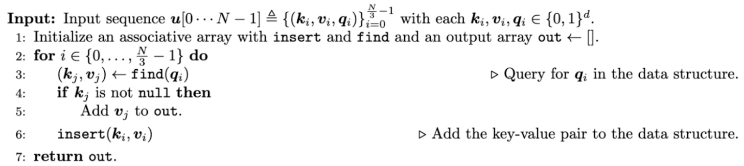
Unfortunately, converting this algorithm to a circuit requires massive $\Omega(N)$ depth of BaseConv in sequence length $N$.

We also came up with a more efficient parallel arithmetic circuit by drawing inspiration from the parallel binary search algorithm, which has $O(\log N)$ depth (Algorithm 10). This allows us to obtain a tighter upper bound for BaseConv and MQAR. Given the equivalence between BaseConv and arithmetic circuits, we could conclude a BaseConv model with $\tilde{O}(Nd)$ parameters and $\tilde{O}(1)$ layers can solve MQAR!

So this is awesome, we have this single powerful BaseConv tool!! Why don’t we just do everything with this? It’s easy to reason about! The issue is: we're still losing poly-log factors on the depth in our bound (recall $\tilde{O}()$ hides poly-log factors) :( While poly-log is relatively tight in theory, in ML architectures, we pay a lot if the depth is too large — it makes things hard to optimize. We really want to know if we can solve MQAR in $O(1)$ layers, like we can do for attention.

Can we do better?

Lower bound for BaseConv and MQAR

Unfortunately, we find can't get $O(1)$ layers with BaseConv :( We show a lower bound on the depth that depends on $N$.

Recapping the situation for one-hot encodings. In our toy constructions in Part 2, we had used one-hot encodings for each token in the sequence. We showed both Attention and BaseConv could solve MQAR with these encodings, but the size of the one-hot encoding is $d=N$, which is much too large.

Expand to recap attention and BaseConvs's one-hot encoding solutions again

Here we describe the Part 2 intuition with math notation :)

We will assume that our input matrix $x\in\{0,1\}^{N\times d}$ uses 1-hot encoding, i.e. each row is a standard basis vector in $\{0,1\}^n$ (note that this implies $d=N$). Note that the attention-query-key inner product, $A[i,j]=\langle Q[i,:],K[j,:]\rangle$, is $1$ if $Q[i,:]=K[j,:]$ and $0$ otherwise (note that we crucially used the fact that each row is 1-hot encoded here). $A$ tells us the positions of matching tokens in MQAR. Given the matching MQAR-key tokens, we want to output the corresponding MQAR-value, so we can let our attention-values be $V = (S \cdot x)$, where $S$ a matrix that shifts entries forwards by one position. We need to use ``positional encodings'' to implement the shift. We can compute $A \cdot V$ to solve the MQAR problem. Visualize this construction.

Moving on to BaseConv, note that all of the above operations for attention are polynomial operations yielding an arithmetic circuit of size $O(N^3)$ and $O(1)$ to solve the MQAR problem. This is because the circuit size is $O(N^2d)$ but we also have $d=n$, so $O(N^3)$ overall. If we use our arithmetic circuit equivalency theorem then we can get an $\tilde{O}(1)$ layer BaseConv implementation with $\tilde{O}(N^3)$ parameters. In other words, for 1-hot-encoded inputs there is no difference between Attention and BaseConv: both can solve MQAR in $O(1)$ layers! However, 1-hot encodings require model dimension to scale with sequence length $N$!

We want more compresssed representations in ML... Things get interesting if we use a more compressed representation. For example, consider the case when $d=\log_2{|C|}$ for vocab $C$. Here we can still use Attention to solve MQAR in $O(1)$ layers. This is because we have that $Q[i,:]=K[j,:]$ (for our $QK^T$ inner products) iff and only if $\langle Q[i,:],K[j,:]\rangle=d$. The latter is obtained with a “threshold” functionality, provided a linear map+ReLU or Softmax/other non-polynomial activation functions. The rest of the Attention construction remains the same.

However, in BaseConv, it is not possible to implement the above threshold “trick” with $O(1)$ layers. In fact, we prove a lower bound in the even simpler case of checking if two vectors $y,x \in \{0,1\}^{\log{|C|}}$ are equal (when $x,y \in C$). The basic takeaway from our proof ends up being that to represent equality exactly, we need a polynomial of degree $d$, but $O(1)$ layer BaseConv can only represent constant degree polynomials.

Note that this argument was tied to a specific encoding of $x$, but are also able to show that regardless of how $x$ is encoded, with $d\le 2^{(\log{N})^{1-\epsilon}}$, a BaseConv model requires the number of layers to solve MQAR to scale with $N$.

Expand for an overview of the proof of this result.

This proof invokes the index problem. The index problem has two agents, Alice and Bob, where Alice has a string $x \in {0, 1}^n$ and Bob has an index $i \in [n]$. The goal for the players is to output the $i^{th}$ entry: $x_i$. We also require the communication to be one-way: only Alice is allowed to send a single message to Bob and Bob needs to output the answer. We reduce MQAR to the index problem (described in Part 4).

1. Properties of BaseConv First we note that an $L$ layer BaseConv model that solves AR on input $x\in\mathbb{R}^{N\times d}$ is equivalent to a polynomial on $Nd$ variables (one corresponding to each entry in the matrix $x$) and has degree at most $2^L$. ⁵ Recall each BaseConv layer is the same as a polynomial of degree at most $2$ -- composing $L$ such layers gives us a polynomial of degree at most $2^L$.

2. We next invoke the index problem. Alice has the input $a=(1,x_1,\dots,n,x_n)$ (encoded as a matrix in $\mathbb{R}^{(N-1)\times d}$) and Bob has the input $b= i \in [n]$ (encoded as a vector in $\mathbb{R}^d$). If there exists an $L$ layer BaseConv model to solve AR, then there exists a polynomial $P(a,b)$ of degree at most $2^L$ that outputs $x_i$. Alice knows everything except $b$. She can substitute her values $a$, to get a polynomial $Q_a(Z)=P(a,Z)$, where $Z$ has $d$ variables as placeholders for Bob’s input and still, the degree of $Q(Z)\le \deg(P)\le 2^L$. Alice sends Bob the coefficients of $Q_a(Z)$ and Bob outputs $Q_a(b)=P(a,b)=x_i$.

3. Lower bound Note that by the lower bound of the index problem, we can conclude that the number of bits Alice needs to encode all the coefficients is $\Omega(N)$. Since $Q(Z)$ is a $d$-variate polynomial of degree at most $2^L$, it has at most $d^{2^L}$ coefficients. If $B$ is the number of maximum number of bits we need to represent any of these coefficients, we have: $B \cdot d^{2^L} \geq \Omega(N)$.

   Using the fact that all of the original parameters in BaseConv model use $O(\log{N})$ bits (as well as the fact that $d\le 2^{(\log{N})^{1-\epsilon}}$), a little bit of algebraic manipulation gives us our claimed lower bound of

$L\ge \Omega\left(\epsilon\cdot\log\log{N}\right)$.

Linear attention and MQAR

We have seen that Transformers can represent MQAR in constant model width and layers, independent of the sequence length $N$, and the scaling needed for gated convolutions to solve MQAR is undesirable.Can we mimic Transformers without the quadratic scaling in sequence length? Enter linear attention models! These retain input-dependent mixing, making it easy to compare tokens in the sequence unlike convolutions, and give nice efficiency properties (sub-quadratic training and constant inference).

We love polynomials In spirit of our polynomial view of efficient architectures, we consider using a natural option for the feature map, a polynomial approximation to the attention exponential function following Zhang et al., 2024. Recall the Taylor approximation of $\exp(x)$:

$\exp(x) = 1 + x + \frac{x}{2!} + … + \frac{x^t}{t!} …$

Let’s let $\otimes$ represent an outer product operation and let the linear attention feature map, $\phi($\cdot$): \mathbb{R}^{N \times d’} \rightarrow \mathbb{R}^{N \times D}$, be the Taylor polynomial for $\exp$ following Zhang et al., 2024:

$\phi(q) = \mathrm{Concatenation}(1, q, (q \otimes q)/2!,…)$

$\phi(k) = \mathrm{Concatenation}(1, k, (k \otimes k)/2!, …)$

Elementwise multiplying $\phi(q)$ and $\phi(k)$, we get for $q, k \in \mathbb{R}^{N \times d’}$: $\exp(qk) = \phi(q)\phi(k) = \mathrm{Concatenation}(1, qk, qqkk/2!,…)$

While we would need infinite terms (i.e., an infinite dimension tensor and amount of GPU hardware memory consumption) to exactly represent attention’s $\exp{qk}$, we find that roughly order-$2$ (feature dimension $D = 1 + d’ + d’^2$) seems to be empirically effective given the range of values that $q$ and $k$ fall into in large language modeling experiments.

Varying values of $d’$ changes the amount of meory (size of $h_t$) the model uses. While arithmetic circuit complexity typically focuses on the total size and depth of the circuit computing polynomials, we also care about the amount of external memory a model uses to produce an answer from a hardware efficiency perspective. Keeping track of the memory starts to fall into the communication complexity model of computation, bringing us to our final section.

---

Part 4: Memory-limited learning

Efficient LMs seeks to reduce the memory requirement relative to Transformers, which require massive “KV”-caches that grow in input length.

Expand to recap the recurrent memory use by architecture!

Let’s briefly review the total state size (GPU memory consumption) $s$ by different architectures as they processes an $x \in \mathbb{R}^{N \times d}$ input (see Appendix E.2 for more discussion).

• Attention: the size of the KV cache ($h_{K}$ and $h_{V}$) described above is: $s = 2 \times d \times N$.
• Linear attention: the state size is determined by $h_t$ as discussed above: $s = dD$, for feature dimension $D$ and model dimension $d$.
• Gated convolution (H3): the state is determined by the number of heads $d_{state}$: $s = d \times d_{state}$.

Specifically, note the efficient Transformer alternatives seek to use external memory that’s independent of sequence length $N$.

Autoregressive language modeling should remind you of one-pass streaming algorithms. In this vein, our theoretical analysis of the memory-efficient LMs invokes a prior lower bound result for the index problem in the one-pass streaming setting: the one-way randomized communication complexity of the index problem for a n-length input bit string is $\Omega(n)$.

Index problem. The index problem has two agents, Alice and Bob, where Alice has a string $x \in {0, 1}^n$ and Bob has an index $i \in [n]$. The goal for the players is to output the $i^{th}$ entry: $x_i$. We also require the communication to be one-way: only Alice is allowed to send a single message to Bob and Bob needs to output the answer.

There is a pretty straightforward reduction from indexing to MQAR (and in fact to the simpler version AR where the query comes at the end). Specifically given the input $x\in\{0,1\}^n$ and $i\in [n]$, the corresponding input to AR is (a sequence; index pair): $1,x_1,\dots,j,x_j,\dots,n,x_n;i$. Note that if a model solves this AR instance, then it should match $i$ to the earlier occurrence of $i$ and output $x_i$.

Recurrent models and MQAR. We can easily conclude that any recurrent model $\mathcal{M}$ that solves MQAR requires the state size to be at least $\Omega(N)$ bits. To show this, suppose Alice runs $\mathcal{M}$ on the portion of the AR input above she has (i.e. $1,x_1,\dots,j,x_j,\dots,n,x_n$) and sends the final state $h_{N-1}$ to Bob, who using the state $h_{N-1}$ and his input $i$ can run $\mathcal{M}$ to output the input value at position $i$. Since we have a lower bound for the index problem, this would present a contradiction and we conclude $\Omega(N)$ bits are required.⁶

Maybe all hope is not lost! Our subsequent work designs multi-pass recurrent models, which can use less memory than autoregressive models depending on the order of information in the input sequences.

---

Part 5: Tying the theory to experiments!

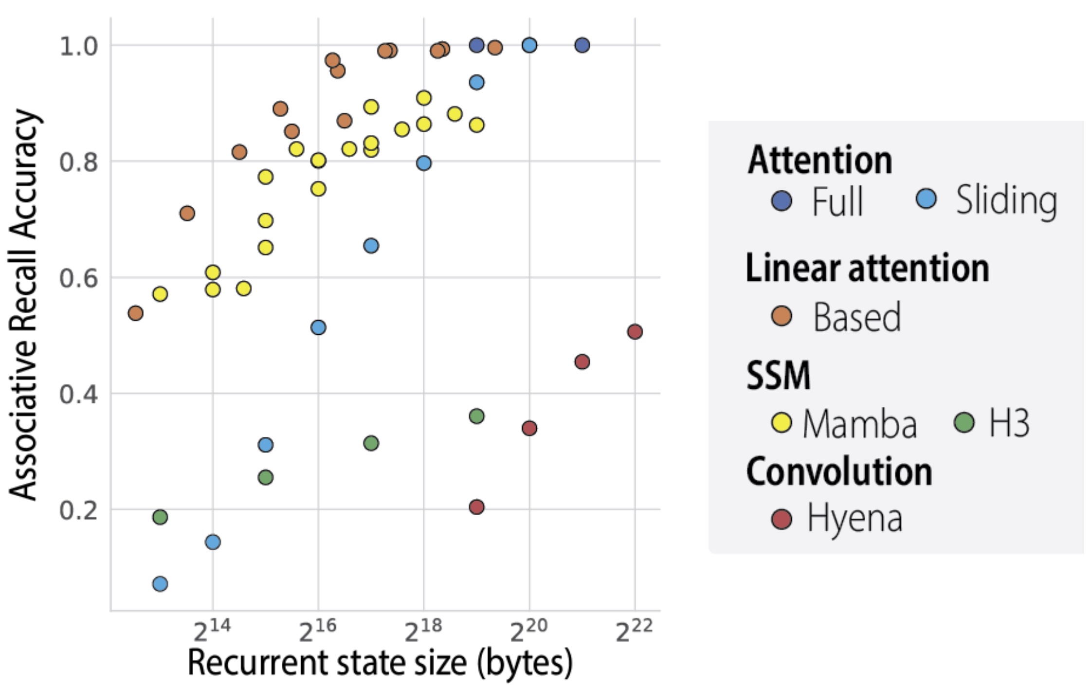
We evaluate several efficient LMs, from the architecture classes discussed above, on the MQAR problem. We vary the recurrent state size, or amount of memory each architecture uses during inference, on the $x$-axis.

We can see the theoretical scaling results reflected in the figure below.

1. Attention baseline Sliding window attention is a natural input-dependent and fixed-memory architecture. As we traverse the window size (memory use), it faces a stark quality tradeoff.
2. Input independent convolutions Gated convolutions (H3, Hyena) falle below the a (sliding window) attention baseline.
3. Input dependent Input-dependent mixers (Based linear attention, Mamba’s selective SSMs) expand the Pareto frontier relative to attention!
4. Memory limits All these recurrent LMs face a memory vs. recall-quality tradeoff. Some models are better than others at using their alotted memory.

You can find more discussion of our empirical results in our prior blogposts and try out our MQAR synthetic here: https://github.com/HazyResearch/zoology. We used our insights to design new LM architectures.

Postscript: Related Works!

If you're interested in this line of work, we've compiled a quick reading list of works on complexity and language models to check out. This is a relatively biased list, please reach out if you have more pointers!

Expand for the related works discussion

Works related to arithmetic circuits and language models:

• A Two-pronged Progress in Structured Dense Matrix Vector Multiplication: Our initial work on structured matrices. The most relevant result on the equivalence of linear arithmetic circuit complexity of $Wx$ and sparse decomposition of $W$ is in Appendix B.
• Kaleidoscope: An Efficient Learnable Representation For All Structured Linear Maps: Proves any (small depth) arithmetic circuit for $Wx$ can be converted into a decomposition of $W$ into structured sparse matrices with only a poly-log loss in parameters. The structured matrices are Butterfly matrices that arise naturally in FFT and lead to a differentiable family of matrices.
• Arithmetic Circuits, Structured Matrices and (not so) Deep Learning: A survey that covers the above two results and puts them in context of the constraints imposed by deep learning. If you do not have much background in deep learning, this could be a good starting point.
• Monarch: Expressive Structured Matrices for Efficient and Accurate Training: This paper proposed Monarch matrices that inherit the nice expressivity properties of Butterfly matrices but are also hardware friendly. In addition, there is a simple solution to the "projection" problem– given an arbitrary matrix, find the closest Monarch matrix in the Frobenius norm.
• Monarch Mixer: A Simple Sub-Quadratic GEMM-Based Architecture: The above work showed how to replace the MLP layer with structured matrices. This paper showed how they can be used to replace Attention layer as well (there is a bunch of polynomial goodness in the appendices to show that these can be implemented in a causal manner).
• On The Computational Complexity of Self-Attention Attention requires quadratic runtime in the worst-case assuming SETH.
• Zoology: Measuring and Improving Recall in Efficient Language Models: Introduced the MQAR problem, the BaseConv architecture and showed how BaseConv can simulate any (small depth) arithmetic circuits (beyond linear arithmetic circuits from Kaleidoscope) with only a poly-log loss in parameters. Simple linear attention language models balance the recall-throughput tradeoff: The theory results are mostly on proving limitations of BaseConv using connections to communication complexity.
• Just read twice: Closing the recall gap for recurrent language models: The theory explores linear recurrent models in the multi-pass setting, whereas most of the work on sub-quadratic architectures focuses on causal single-pass streaming language modeling.

State space models:

• HiPPO: Recurrent Memory with Optimal Polynomial Projections: Formulated the online functional approximation problem and connected it to orthogonal polynomials. Combining Recurrent, Convolutional, and Continuous-time Models with Linear State Space Layers: Connected linear state space models to HiPPO and explicitly pointed out the advantages of its recurrent and convolutional views.
• Efficiently Modeling Long Sequences with Structured State Spaces introduced the exciting S4 state space model based architecture! and How to Train Your HiPPO: State Space Models with Generalized Orthogonal Basis Projections provides some more theoretical grounding for choices in S4.
• Mamba: Linear-Time Sequence Modeling with Selective State Spaces State space models with data dependent state space model parameters! This has created lots of buzz!
• Transformers are SSMs: Generalized Models and Efficient Algorithms Through Structured State Space Duality: A nice theoretical framework that connects works on state space models to those in linear attention.

Connections to other “traditional” computation models There is a rapidly growing body of work connecting language model architectures to well studied models of computation (other than arithmetic circuits, e.g. boolean circuits) mainly with the goal of showing limitations of these models. Since this body of work is slightly orthogonal to this blog post, we’ll just give a biased sample below:

• Log-precision Transformers are in $TC^0$; With infinite precision, Transformers are as powerful as Turing machines
• Log-precision Transformers are in a (slight) generalization of first order logic statements
• A strong dichotomy result on runtime of Attention based on whether the precision is sub-logarithmic or not.
• Commonly used instantiations of State Space Models are in $TC^0$ as well!

Takeaways and future questions

We’ve had a ton of fun playing with MQAR and trying to build efficient LMs that solve it more efficiently over the past while. Overall, we hope the polynomial view of efficient LMs helps you reason about key ingredients like input-dependent sequence mixing and managing the quality-efficiency tradeoffs around recurrent state size.

A couple of questions for that might be interesting to think about:

1. What are other “toy tasks”, like MQAR, that both are empirically meaningful and enable theoretical analysis? Perhaps not only for the sequence mixer. Work from [11] shows that both Transformers and SSMs struggle with certain capabilities like state tracking. Can we better understand when state tracking is important in language modeling with simple synthetics?
2. We also don’t use the full power of BaseConv to prove our results (we largely instantiate a few types of convolution kernels, like shift kernels). What are the minimal sufficient representations for the capabilities we need?
3. Our results show that there exists BaseConv models that exactly solve MQAR. However, we do not have any proof that running Gradient Descent with MQAR will converge to a BaseConv model that can solve MQAR. It would be very nice to prove that this is indeed the case. As a first step, it would be nice to present any provable fast learning algorithm that given test data from MQAR learns a BaseConv model that solves the problem.

Please feel free to reach out to us: simran@cs.stanford.edu and eyuboglu@stanford.edu.