Dec 5, 2020 · 13 min read
HiPPO: Recurrent Memory with Optimal Polynomial Projections
Albert Gu*, Tri Dao*, Stefano Ermon, Atri Rudra, and Chris Ré
Many areas of machine learning require processing sequential data in an online fashion. For example, a time series may be observed in real time where the future needs to be continuously predicted, or an agent in a partially-observed environment must learn how to encode its cumulative experience into a state in order to navigate and make decisions. The fundamental problem in modeling long-term and complex temporal dependencies is memory: storing and incorporating information from previous time steps.
However, popular machine learning models suffer from forgetting: they are either built with fixed-size context windows (e.g. attention), or heuristic mechanisms that empirically suffer from from a limited memory horizon (e.g., because of "vanishing gradients").
This post describes our method for addressing the fundamental problem of incrementally maintaining a memory representation of sequences from first principles.

Many areas of machine learning require processing sequential data in an online fashion. For example, a time series may be observed in real time where the future needs to be continuously predicted, or an agent in a partially-observed environment must learn how to encode its cumulative experience into a state in order to navigate and make decisions. The fundamental problem in modeling long-term and complex temporal dependencies is memory: storing and incorporating information from previous time steps.
However, popular machine learning models suffer from forgetting: they are either built with fixed-size context windows (e.g. attention), or heuristic mechanisms that empirically suffer from from a limited memory horizon (e.g., because of "vanishing gradients").
This post describes our method for addressing the fundamental problem of incrementally maintaining a memory representation of sequences from first principles. We will:
-
find a technical formulation of this problem that we can analyze mathematically, and derive a closed-form solution with the HiPPO framework
-
see that our method can be easily integrated into end-to-end models such as RNNs, where our framework both generalizes previous models, including the popular LSTM and GRU, and improves on them, achieving state of the art on permuted MNIST, a popular benchmark for long-range memory.
-
show how insights from the framework reveal methods with distinct theoretical properties -- we highlight a particular model HiPPO-LegS, which is computationally efficient, provably alleviates vanishing gradients, and is the first known method to display "timescale robustness"!
Our paper was accepted to Neurips 2020 as a Spotlight, and our code is publically available with PyTorch and Tensorflow implementations.
Online Function Approximation: A Formalism for Incremental Memory Representations
Our first insight is to move from discrete-time to the continuous-time setting, which is often easier to analyze theoretically. We ask the following very natural question: given a continuous function (in one dimension) , can we maintain a fixed-size representation at all times such that optimally captures the history of from times to ?
However, this problem is not fully well-defined yet -- we need to specify:
-
Quality of approximation: What is the "optimal approximation" of the function's history? We need to specify a measure (or weight function) that tells us how much we care about every time in the past.
-
Basis: How can we compress a continuous function into a fixed-length vector? We can project the function onto a subspace of dimension and store the coefficients of its expansion in any basis. For simplicity, we will assume that we are working with the polynomial basis throughout this post.
Intuitively, we can think of the memory representation as being the coefficient vector of the optimal polynomial approximation to the history of .
The HiPPO Framework (High-Order Polynomial Projection Operator)
Notice that given a measure (and assuming the polynomial basis), the online function approximation problem is now fully specified!measure That is, given any input function , the desired coefficient vectors , which are our desired memory representation, are completely defined. The question remains -- how do we calculate them?
The HiPPO framework formalizes this problem and provides machinery to compute the solution. Although the desired coefficients are rather abstractly defined as the implicit solution to an approximation problem, there is amazingly a closed-form solution that's easy to compute. We'll leave the technical details to the full paper, but we'll note that they leverage classic tools from approximation theory such as orthogonal polynomialsop. In the end, the solution takes on the form of a simple linear differential equation, which is called the HiPPO operator:
In short, the HiPPO framework takes a family of measures, and gives an ODE with closed-form transition matrices . These matrices depend on the measure, and following these dynamics finds the coefficients that optimally approximate the history of according to the measure.
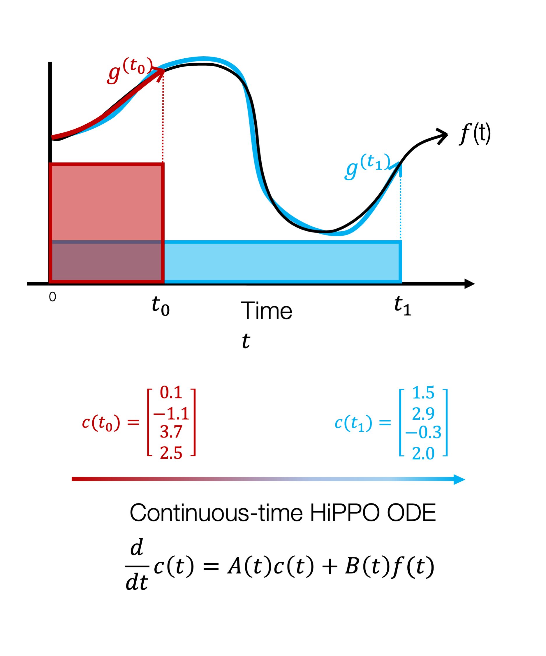
Figure 1: The HiPPO Framework. An input function (black line) is continually approximated by storing the coefficients of its optimal polynomial projections (colored lines) according to specified measures (colored boxes). These coefficients evolve through time (red, blue) according to a linear dynamical system.
Instantiations of HiPPO
Figure 2 shows some concrete examples of HiPPO. We show two of the simplest family of measures, based off uniform measures. The translated Legendre measure on the left uses a fixed-length sliding window; in other words, it cares about recent history. On the other hand, the scaled Legendre measure uniformly weights the entire history up to the current time. In both cases, the HiPPO framework produces closed-form formulas for the corresponding ODEs which are shown for completeness (the transition matrices are actually quite simple!).
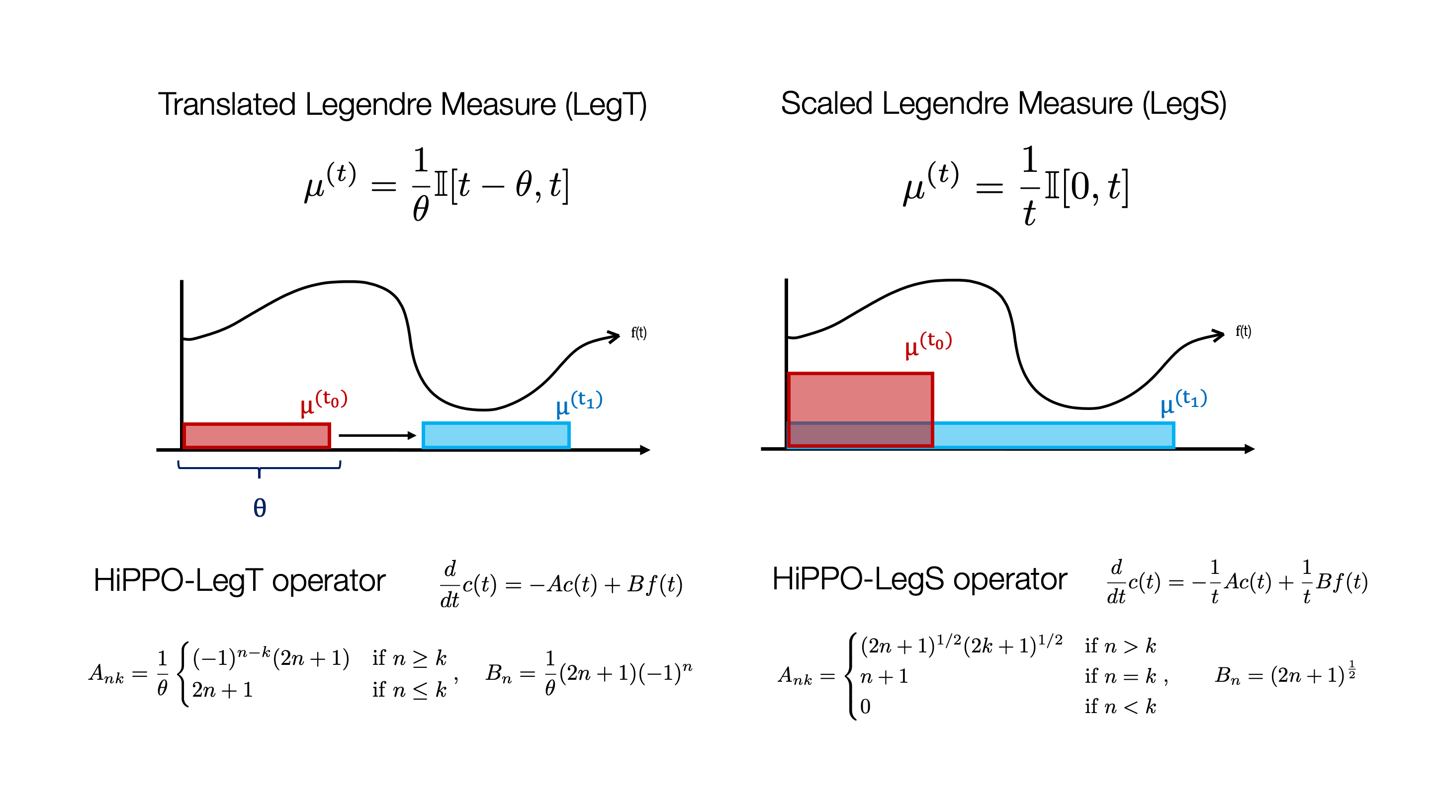
Figure 2. Examples of simple measures and their corresponding HiPPO operators. The Translated Legendre Measure uniformly weights the past (a hyperparameter) units of time, while the Scaled Legendre Measure uniformly weights all history.
From continuous-time to discrete-time
There is one more detail called discretization. By using standard techniques for approximating the evolution of dynamical systems, the continuous-time HiPPO ODE can be converted to a discrete-time linear recurrence. Additionally, this step allows extensions of HiPPO to flexibly handle irregularly-sampled or missing data: simply evolve the system according to the given timestamps.
For the practitioner: To construct a memory representation of an input sequence , HiPPO is implemented as the simple linear recurrence where the transition matrices have closed-form formulas. That's it!
Hippos in the wild: integration into ML models
At its core, HiPPO is a simple linear recurrence that can be integrated into end-to-end models in many ways. We focus on a recurrent neural network (RNN) due to their connection to dynamics systems involving a state evolving over time, just as in HiPPO. The HiPPO-RNN is the simplest way to perform this integration:
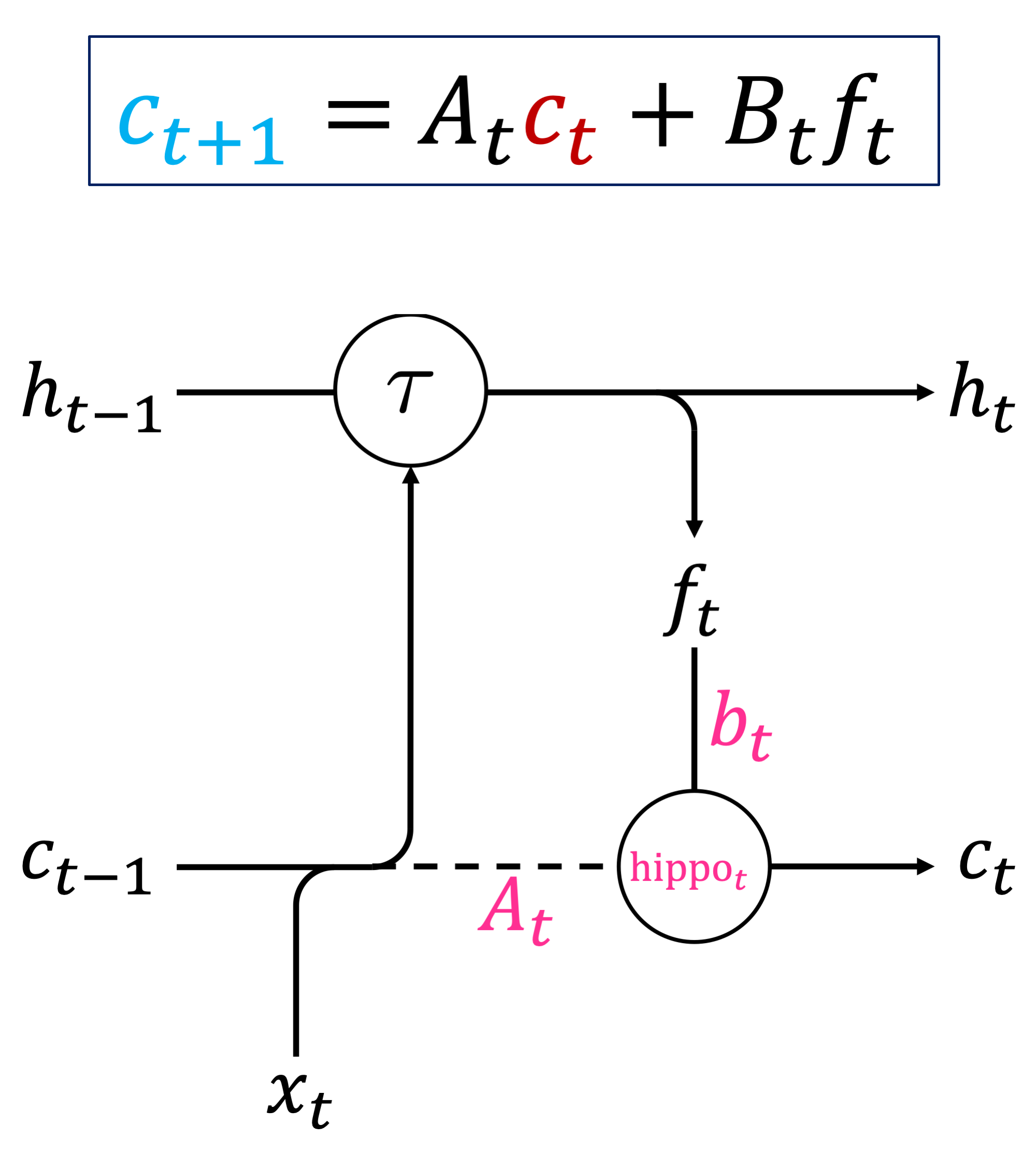
Figure 3. (Top) HiPPO on discrete sequences has the form of a simple linear recurrence. (Bottom) The HiPPO-RNN cell diagram.
-
Start with a standard RNN recurrence that evolves a hidden state by any nonlinear function given the input
-
Project the state down to a lower dimension feature
-
Use the HiPPO recurrence to create a representation of the history of , which is also fed back into
Special cases of the HiPPO-RNN
Those familiar with RNNs may notice this looks very similar to cell diagrams for other models such as LSTMs. In fact, several common models are closely related:
-
The most popular RNN models are the LSTM and GRU, which rely on a gating mechanism. In particular, the cell state of an LSTM performs the recurrence , where are known as the "forget" and "input" gates. Notice the similarity to the HiPPO recurrence . In fact, these gated RNNs can be viewed as as a special case of HiPPO with low-order (N=1) approximations and input-dependent discretization! So HiPPO sheds light on these popular models and shows how the gating mechanism, which was originally introduced as a heuristic, could have been derived.
-
The HiPPO-LegT model, which is the instantiation of HiPPO for the translated Legendre measure, is exactly equivalent to a recent model called the Legendre Memory Unitlmu. Our proof is also much shorter, and just involves following the steps of the HiPPO framework!
Elephants Hippos never forget
Let's take a look at how these models perform on benchmarks. First, we test if HiPPO solves the problem it was designed to -- online function approximation. Figure 4 shows that it can approximate a sequence of a million time steps with good fidelity. Keep in mind that this works while processing the function online with a limited budget of hidden units; it could have reconstructed the partial function at any point in time.
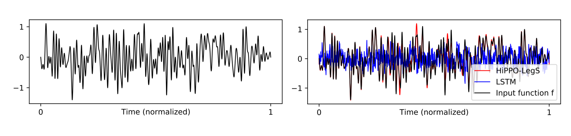
Figure 4. (Left) a band-limited white noise function, sampled to a sequence of length 1000000. (Right) Reconstruction of the approximate function after processing the sequence with 256 hidden units. HiPPO closely matches the original function (MSE 0.02), while the LSTM produces random noise (MSE 0.25).
Second, we test on the standard Permuted MNIST benchmark, where models must process the input image one pixel at a time and output a classification after consuming the entire sequence. This is a classic benchmark for testing long-term dependencies in sequence models, since they must remember inputs from almost 1000 time steps ago.
Multiple instantiations of our HiPPO framework, including the HiPPO-LegS and HiPPO-LegT models described above, set state-of-the-art over other recurrent models by a significant margin, achieving 98.3% test accuracy compared to the previous best of 97.15%. In fact, they even outperform non-recurrent sequence models that use global context such as dilated convolutions and transformers. Full results can be found in Tables 4+5.
Timescale Robustness of HiPPO-LegS
Lastly, we'll explore some theoretical properties of our most interesting model, corresponding to the Scaled Legendre (LegS) measure. As motivation, the discerning reader may be wondering by this point: What's the difference between different instantiations of HiPPO? How does the measure influence the model? Here are some examples of how intuitive interpretation of the measure translates into theoretical properties of the downstream HiPPO model:
-
Gradient bounds: Since this measure says that we care about the entire past, information should propagate well through time. Indeed, we show that gradient norms of the model decay polynomially in time, instead of exponentially (i.e. the vanishing gradient problem for vanilla RNNs).
-
Computational efficiency: The transition matrices actually have special structure, and the recurrence can be computed in linear instead of quadratic time. We hypothesize that these efficiency properties are true in general (i.e., for all measures), and are related more broadly to efficiency of orthogonal polynomials and their associated computations (e.g. [link to SODA paper])
-
Timescale robustness: Most interestingly, the scaled measure is agnostic to how fast the input function evolves; Figure 5 illustrates how HiPPO-LegS is intuitively dilation equivariant.
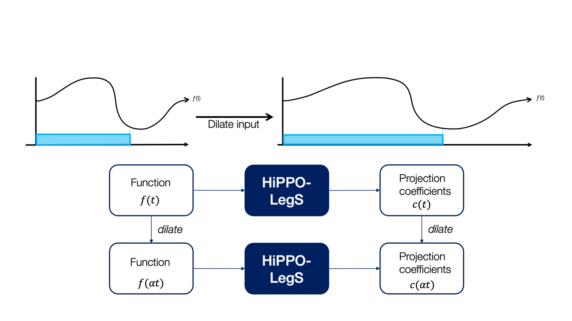
Figure 5. (Top) Since the scaled Legendre measure stretches through time, intuitively, dilating an input function should not change the projections. (Bottom) A commutative diagram illustrating how the HiPPO-LegS operator is equivariant to time dilation.
The table shows results on a trajectory classification dataset with distribution shift between the training and test sequences (i.e., arising from time series being sampled at different rates at deployment); HiPPO is the only method that can generalize to new timescales!
| Generalization | LSTM | GRU-D | ODE-RNN | NCDE | LMU | HiPPO-LegS |
|---|---|---|---|---|---|---|
| 100Hz -> 200Hz | 25.4 | 23.1 | 41.8 | 44.7 | 6.0 | 88.8 |
| 200Hz -> 100Hz | 64.6 | 25.5 | 31.5 | 11.3 | 13.1 | 90.1 |
Conclusion
-
The problem of maintaining memory representations of sequential data can be tackled by posing and solving continuous-time formalisms.
-
The HiPPO framework explains several previous sequence models as well as produces new models with cool properties.
-
This is just the tip of the iceberg - there are many technical extensions of HiPPO, rich connections to other sequence models, and potential applications waiting to be explored!
Try it out
PyTorch and Tensorflow code for HiPPO are available on GitHub, where the HiPPO-RNNs can be used as a drop-in replacement for most RNN-based models. Closed-form formulas and implementations are given for the HiPPO instantiations mentioned here, and several more. For more details, see the full paper.
Footnotes
- A measure induces a Hilbert space structure on the space of functions, so that there is a unique optimal approximation - the projection onto the desired subspace.↩
- Examples of famous orthogonal polynomials include the Chebyshev polynomials and Legendre polynomials. The names of our methods, such as LegS (scaled Legendre), are based off the orthogonal polynomial family corresponding to its measure.↩
- The way we integrate the HiPPO recurrence into an RNN is slightly different, so the full RNN versions of the HiPPO-LegT and Legendre Memory Unit (LMU) are slightly different, but the core linear recurrence is the same.↩