Jul 1, 2020 · 11 min read
Addressing Hidden Stratification: Fine-Grained Robustness in Coarse-Grained Classification Problems
Nimit Sohoni, Jared Dunnmon, Geoffrey Angus, Albert Gu, and Chris Ré
The classes in classification tasks are often composed of finer-grained subclasses. Models trained using only the coarse-grained class labels tend to exhibit highly variable performance across different subclasses. Moreover, the subclasses are often unknown ahead of time, making it difficult to identify and reduce such performance gaps. This hidden stratification problem can be critical in applications such as medical imaging and algorithmic fairness, where the costs of different types of mistakes are not equal.
We propose a framework to address hidden stratification that combines representation learning, unsupervised clustering, and robust optimization to automatically identify the subclasses and train models with better worst-case subclass performance—without requiring prior knowledge of the subclasses! In this way, our framework allows ML practitioners to find poorly-performing subclasses and improve performance on them, without needing to resort to expensive re-labeling of the data.
What is Hidden Stratification?
In many real-world classification tasks, each labeled class (or superclass, for clarity) is a broad category that consists of multiple distinct subclasses. For example, when classifying between images of cats and dogs, subclasses of the “dog” class might be different breeds: Labradors, Chihuahuas, etc., and likewise subclasses of the “cat” class might be Persian, Siamese, etc. Because models are typically trained to maximize global metrics like average performance, they often underperform on important subclasses. For instance, some cat breeds may look more “doglike” than others, making them harder to classify; or, a breed may be underrepresented in the dataset, leading to worse generalization error on that breed. This phenomenon, which we call hidden stratification, can lead to skewed assessments of model quality, resulting in unexpectedly poor performance when models are deployed in production.

Figure 1. A dog, a cat, and a cat that looks kind of like a dog.
For a less frivolous—and much more concerning—example, a medical imaging model trained to classify between benign and abnormal pathologies might achieve good average performance, yet consistently mislabel a rare but critical disease subclass as “benign” (Dunnmon et al., 2019). A key obstacle to correcting these undesirable effects is that subclass labels for the data are often unavailable, even when the superclass labels are abundant. For instance, it may be more expensive to collect more specific subclass labels compared to the coarser-grained superclass labels—most human annotators can quickly label cat vs. dog images, but one would need more specialized knowledge, and time looking at the image, to identify particular breeds. More fundamentally, the subclass identities might even be unknown a priori.
When the subclasses are not labeled, it’s hard to even recognize whether a model performs poorly on some subclasses, let alone correct for this! In high-risk applications like medical imaging, this kind of uncertainty can be unacceptable. Can we somehow ensure good performance across all subclasses, without being given any information about them?
In this post, we focus on understanding hidden stratification, and using the insights we gain to mitigate it—even when subclass labels are unavailable!
- First, we present and analyze a simple statistical model that explains one mechanism by which hidden stratification can occur.
- We use the insight gained from our analysis to correct for hidden stratification in this setting. We present a two-stage framework to (1) estimate the subclasses (via clustering) and then (2) improve performance on these estimated subclasses (via robust optimization); we show that this approach can help close performance gaps between subclasses. Our results show that our approach has potential–but there’s still a lot more to explore.
Why Does Hidden Stratification Occur?
To understand why hidden stratification occurs, let’s first look at a simple, concrete example. Consider Fig. 2, in which the goal is to classify between the red and blue “superclasses”; the four circles represent the subclasses. When we train a regularized logistic regression classifier with standard empirical risk minimization (ERM), the resulting decision boundary is the black diagonal line: the classifier pays little attention to the rare subclasses in the lower left and upper right and misclassifies them, even though it attains low average loss.
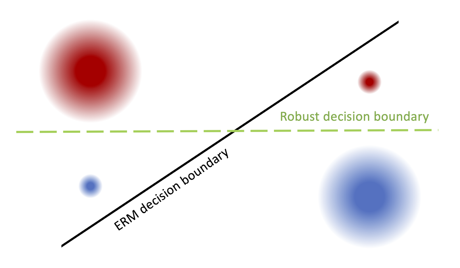
Figure 2. An example of hidden stratification (superclass denoted by color). Dataset imbalance causes rare subclasses (bottom left, top right) to be misclassified by the ERM model, whose decision boundary is in black, whereas the “robust” model, which does best in the worst-case, is the green dashed line.
We’d like to avoid this type of phenomenon, as we are interested in optimizing for robust performance, i.e. the worst-case performance over any subclass. In Fig. 2, the decision boundary that minimizes worst-case subclass loss is the green horizontal line.
Of course, real data rarely looks as simple as Fig. 2. In real datasets, examples are described by multiple attributes, yet often only a subset of these are captured by the human-annotated class labels. We model this data generation and annotation process with the following simple hierarchical generative model (illustrated in Fig. 3). First, a binary "attribute vector" Z is sampled from a distribution p(Z). Each entry Zi is a different attribute, while each unique value of the vector Z represents a different subclass. Then, a latent "feature vector" W is sampled from a distribution conditioned on Z, where W is Gaussian conditioned on Z. Finally, the datapoint X is determined by the latent features W via a mapping X = g(W). Meanwhile, the superclass label Y is a fixed function of a subset of Z1, ..., Zk. Data with the same Y value yet different Z values correspond to different subclasses of a superclass. X and Y are observed, while W and Z are not.
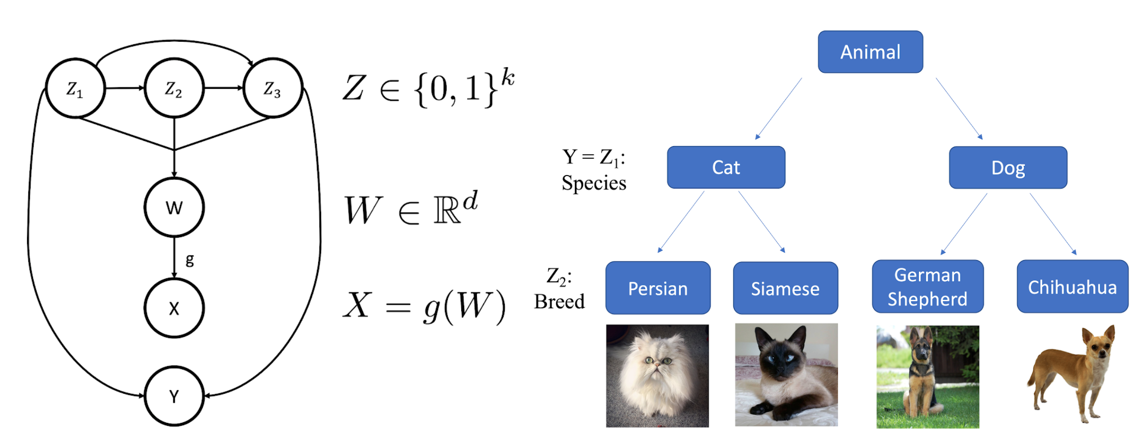
Figure 3. Left: Example illustration of the generative model of hidden stratification; underlying (possibly dependent) attributes Z determine features W and labels Y; W undergoes a transformation g to yield data X. Right: Z = (Z1, Z2) represents both the animal species and breed, while Y only reflects the species.
A key assumption is that the subclasses are “meaningful” in some sense, rather than just arbitrary groups of datapoints. (Requiring the model to perform well on “all possible subsets” of the data is a fairly pessimistic notion; if there’s more structure to the subclasses, we can exploit this!) We model this by the Gaussian assumption on p(W|Z).
The uncaptured axes of variation (corresponding to the “hidden attributes” Zi which do not influence the label Y) can naturally induce hidden stratification, e.g. in the presence of subclass size imbalances. For instance, in feature space, the data distribution p(W) is a mixture of Gaussians, which might look something like Fig. 2. So, even if a model successfully recovers the latent features W from the data X, ERM can still lead to substantial underperformance on certain subclasses when the label annotations are insufficiently fine-grained.
How Do We Solve It?
To mitigate hidden stratification, we introduce a simple two-step procedure. First, we attempt to discover the subclasses using unsupervised clustering. If we can estimate the subclasses well, we can then encourage the model to perform well on these estimated subclasses using robust optimization—optimizing for worst-case rather than average-case performance.
How can we detect the subclasses without labels for them? Intuitively, if we train a sufficiently powerful neural network on the original task, we expect it to learn a meaningful feature representation. If the data approximately follows our generative model, each subclass is described by a different Gaussian in the latent feature space—so clustering in feature space should approximately recover the subclasses! For this to work, the neural network should be powerful enough to approximately “invert” the mapping g from feature vectors to datapoints, and thereby recover the underlying feature space. If not, we can’t expect clustering to work well in general, as illustrated in Fig. 4.
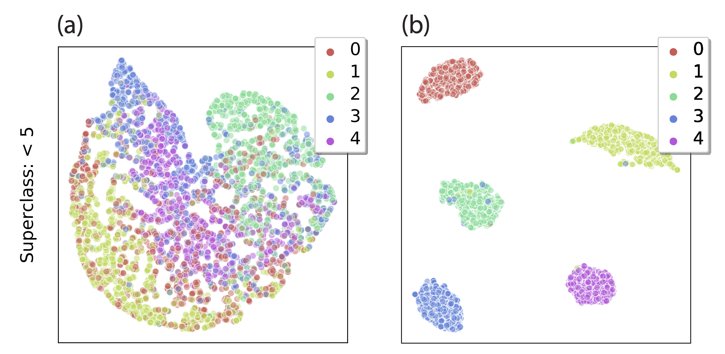
Figure 4. Neural network features for “< 5” superclass on MNIST, with true subclasses indicated by color. The features of a simple convolutional network (LeNet5, right) lead to well-separated subclasses, unlike the features of a fully-connected LeNet 300-100 (left).
Another possible way to obtain a feature representation of the data is to use pretrained image embeddings, such as the recently released BiT embeddings, and cluster the data in this feature space instead. This has the advantage of not having to first train an ERM model on the task—but the downside is that these general image features may not contain relevant task-specific information. In our experiments, we evaluate both approaches.reduction
If the clusters we find approximately correspond to the true subclasses, then inducing good performance across all clusters should encourage good performance across all subclasses. We can do this by simply minimizing the maximum loss across all clusters. We utilize the recent GDRO algorithm (Sagawa et al., 2020) to do this efficiently.
Results
We evaluate our approach on four benchmark tasks: U-MNIST,umnist Waterbirds, CelebA, and the ISIC skin lesion classification task. In Fig. 5, we visualize the recovered clusters and present example images from each cluster. The examples from different clusters are visually distinct, suggesting that the clusters are indeed meaningful. In Table 1, we evaluate our end-to-end method in terms of robust performance. Despite not requiring subclass labels, our end model generally improves upon that of ERM; the robust performance of our model approaches the robust performance of a GDRO model trained using the true subclass labels.
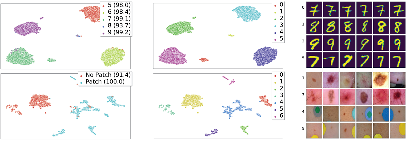
Figure 5. Human-labeled subclasses [with val. set accuracies] visualized in feature space, after UMAP reduction to dimension 2 (left); recovered clusters colored by cluster index (middle); and randomly selected examples from clusters (right). Row 1: MNIST, ≥ 5 superclass; row 2: ISIC, benign superclass.
We find that the approach of training an ERM model and then clustering its activations works well in recovering the subclasses in most cases; however, on the CelebA dataset, clustering pretrained BiT embeddings works significantly better, leading to improved robust performance. In our paper, we provide more detailed comparisons of these two featurization approaches.
| ERM | Ours | GDRO w/annotated subclass labels | |
|---|---|---|---|
| Waterbirds | 60.7 | 83.3 | 90.7 |
| MNIST | 94.2 | 95.7 | 96.8 |
| CelebA | 40.3 | 87.3 | 89.3 |
| ISIC (No-patch) | 92.2 | 91.2 | 92.3 |
| ISIC (Histopathology) | 87.5 | 87.6 | 87.5 |
Table 1. Worst-case subclass performance on the test set (metric is accuracy for MNIST, Waterbirds, and CelebA, and AUROC for ISIC). For ISIC, we report results for both the non-patch subclass and the histopathology subclass; while all methods perform similarly on the non-patch subclass, our method performs best on histopathology examples, as it typically identifies these as a separate cluster. Clustering was done on ERM model representations for all datasets but CelebA, which uses BiT embeddings. Bolded values are best between ERM and our method, both of which do not require subclass labels.
Interestingly, the clusters we discover sometimes correspond to factors of variation that we ourselves were not previously aware of! For example, on U-MNIST we find that, while different digits typically form different clusters as expected, 7’s with a line through the middle (Fig. 5, top right) often also form their own cluster. On ISIC, the task is to classify between benign and malignant skin lesions. Several of the benign examples contain a colorful patch (Fig. 5, lower right), which makes them easy to classify. When we cluster, we find that each cluster is nearly homogeneous (over 97% of either “patch,” or of “no-patch”), even though the training labels do not specify the absence/presence of patches. Further, the benign examples without a patch often separate further into multiple clusters; upon inspection, we found that one of these clusters corresponds to “histopathology” examples – i.e. examples where a biopsy was required to make a diagnosis. Unsurprisingly, model performance on this cluster is the worst of all!
Summary
Our results suggest that our framework is a promising approach to addressing performance gaps between unknown subclasses. This work is just the tip of the iceberg—we look forward to further teasing apart the factors that cause hidden stratification in modern ML tasks, understanding how to obtain better feature representations in order to more accurately identify the subclasses through clustering, and applying our method to broader types of datasets and tasks. We hope that our insights and algorithm will be useful to practitioners in assessing and mitigating hidden stratification in their own applications. Our code is available on GitHub, and our paper (to appear in NeurIPS 2020!) can be found here—we’d love to hear your feedback!
Related Posts
- Improving Medical AI Safety by Addressing Hidden Stratification
- Automating the Art of Data Augmentation (Part IV: New Direction)
Footnotes
- In our experiments, we also apply dimensionality reduction before clustering–see our paper for more details.↩
- U-MNIST is a modified binary classification version of MNIST (the task is to classify digits as “< 5” and “≥ 5”, where the digits 0-9 are the subclasses), with the “8” subclass undersampled, which makes it harder to achieve good performance on this subclass.↩