Nov 13, 2023 · 11 min read
FlashFFTConv: Efficient Convolutions for Long Sequences with Tensor Cores
Convolution models with long filters now have state-of-the-art reasoning abilities in many long-sequence tasks, from long-range language modeling to audio analysis and DNA modeling. But they lag behind the most optimized Transformers in wall-clock time. A major bottleneck is the Fast Fourier Transform (FFT), which allows long convolutions to run in time in sequence length but has poor hardware utilization. We propose FlashFFTConv, a new algorithm for efficiently computing the FFT convolution on GPUs. FlashFFTConv speeds up convolutions by up to 7.93x over PyTorch and achieves up to 4.4x speedup end-to-end. Starting at sequence length 2K, FlashFFTConv starts to match the performance of FlashAttention-v2 – and outperforms it for longer sequences, achieving up to 62% MFU.
Paper: FlashFFTConv: Efficient Convolutions for Long Sequences with Tensor Cores. Daniel Y. Fu*, Hermann Kumbong*, Eric Nguyen, Christopher Ré. arXiv link.
Try it now: https://github.com/HazyResearch/flash-fft-conv
FlashFFTConv: Efficient Convolutions for Long Sequences with Tensor Cores
Over the past few years, we’ve seen convolutional sequence models take the world of long-sequence modeling by storm. From S4 and follow-ups like S5 and DSS, to gated architectures like Monarch Mixer, BiGS, Hyena, and GSS, to hybrid architectures like Mega, H3, and Liquid-S4 – long convolutional models have had a major impact and are here to stay.
These models are exciting because they are sub-quadratic in sequence length – thanks to the FFT convolution algorithm, they can be computed in time in sequence length :
def conv(u, k):
    u_f = torch.fft.fft(u)
    k_f = torch.fft.fft(k)
    y_f = u_f * k_f
    return torch.fft.ifft(y_f)
Compare this against Transformers, which have compute that grows in in sequence length , and you’ve got something that scales better than attention! We’re especially excited about the downstream applications that are being enabled by these new architectures, like audio generation from raw waveforms and DNA modeling directly from base pairs.
But despite this asymptotically better scaling, these convolutions can actually be slower than the most optimized Transformers! That’s because – as is often the case in computer science, the big-O scaling is better, but the constants hiding behind the big-O notation are significant. Why do this work now?
ML workloads have different bottlenecks than traditional FFT workloads, and modern hardware like GPUs has different characteristics than the hardware that was available when traditional FFT algorithms were designed. This necessitates a different approach to the FFT.
We have developed FlashFFTConv, a new algorithm for efficiently computing FFT convolutions on GPUs that builds on a set of insights we’ve been studying over the past two years.
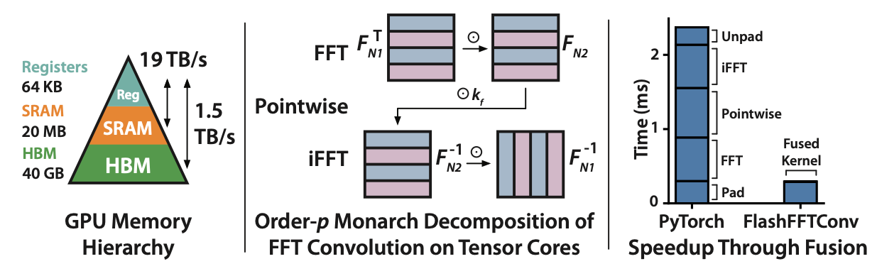
FlashFFTConv uses a Monarch decomposition to fuse the steps of the FFT convolution and use tensor cores on GPUs.
The main insight of our work is that a Monarch decomposition of the FFT allows us to fuse the steps of the FFT convolution – even for long sequences – and allows us to efficiently use the tensor cores available on modern GPUs.
In this rest of this blog post, we’ll go over the key bottlenecks behind the FFT convolution, and then discuss how the Monarch decomposition allows us to overcome those bottlenecks – if we balance the FLOPs and I/O correctly. Then we’ll end with some highlights from our evaluation.
As always, you can check out our paper for more details, such as a deep dive into how FlashFFTConv enables exploration of new sparse primitives for convolutions. Check out our code to try it out yourself – as well as our kernel for the fastest depthwise convolutions for short kernels (7x faster than Conv1D!).
Bottlenecks of the FFT Convolution in ML
If you’re familiar with the FFT, you’re probably asking yourself – Why do we even need a specialized algorithm for the FFT convolution? Didn’t we solve this problem ages ago?
There’s a grain of truth to this – the FFT algorithm has been described as the most important numerical algorithm of our lifetime, and people have been optimizing it for ages. The FFT algorithm that you were taught in class, and the one that you get from YouTube explainers, dates back to 1965 (or 1805 if you go back to Gauss). But this narrative hides a great deal of complexity behind the FFT algorithms that are used in practice, from Bailey’s FFT algorithm, to Winograd FFT, Rader’s algorithm, and many others. The key behind all these developments is that they’re closely tied to the compute and memory paradigms of the day.
For example, there was a time when multiplying numbers was more expensive than adding them -- so the Winograd FFT algorithm tries to minimize multiplication. There’s even a Hexagonal FFT designed for data sampled on hexagonal grids!
So what are the bottlenecks in ML hardware? There are two critical trends to understand, which can you read from two charts:
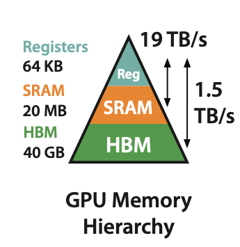
The GPU memory hierarchy, and bandwidth between different layers.
First – there are order-of-magnitude differences in bandwidth between reading from different sections of the GPU memory hierarchy.
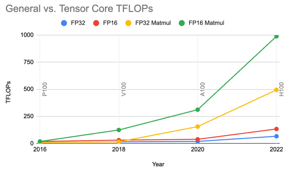
FLOPs available for matmul (green and yellow) compared to general arithmetic (red and blue).
Second – matrix-matrix multiply (the green and yellow lines) is a lot faster than general floating point operations. And the trend is accelerating – matrix-matrix multiply was 8x faster than general arithmetic on V100 in 2018, but is now 16x faster on A100 and H100.
On A100 and H100, multiplying two 16x16 matrices in tensor cores is 16x faster than doing it one operation at a time using general arithmetic operations.
These trends bring two key bottlenecks with them:
- Compute has improved much faster than memory I/O – so I/O is now a major bottleneck.
- Matrix-matrix multiply is significantly faster than general floating point operations.
So what does that mean for FFT algorithms? It’s now much more important to carefully account for I/O than it is to purely count FLOPs, and it’s critical to use matrix multiply operations whenever we can.
Addressing these Bottlenecks with the Monarch Decomposition
In FlashFFTConv, we address these bottlenecks with a Monarch decomposition of the FFT. In brief, the Monarch decomposition allows us to do two things:
- It allows us to break the FFT into matrix-matrix multiply operations, which lets us use tensor cores.
- It allows us to fuse multiple steps of the FFT convolution together, even for long sequences.
Monarch for Matrix-Matrix Multiply
Here’s a simple illustration of the Monarch FFT decomposition:
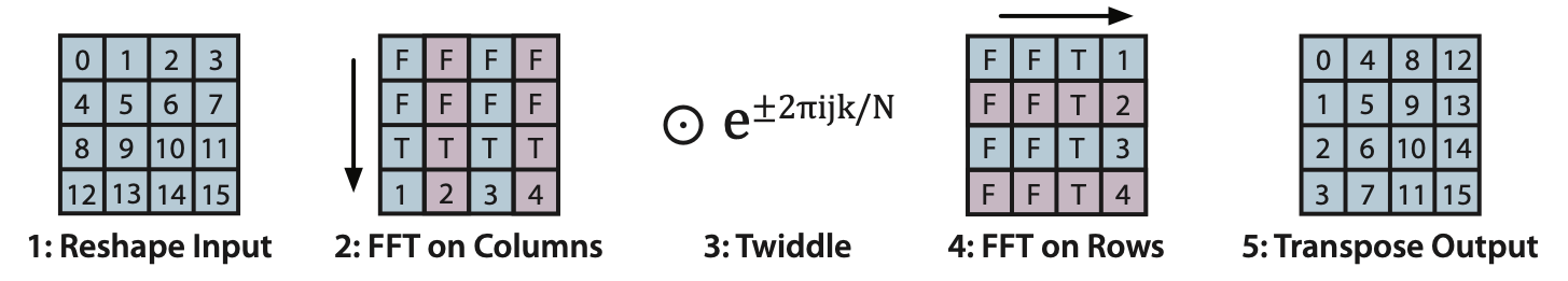
Monarch decomposition of the FFT. Also known as Bailey's FFT, or the four-step FFT.
Given an FFT of length , the Monarch decomposition lets us compute the FFT by reshaping the input into an , compute the FFT on the columns, adjust with the outputs, compute the FFT on the rows, and then transpose the output.
But the FFT operation itself can be expressed as a matrix-matrix multiply operation! So given this mathematical formulation, we can break up the FFT convolution into a series of matrix-matrix multiply operations:
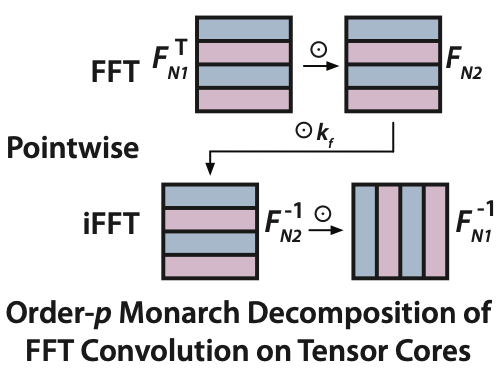
FFT convolution using Monarch decomposition.
What we’re doing here is taking Fourier matrices , computing the FFT over the “columns” or “rows” of the input via matrix-matrix multiply, and adjusting with pointwise operations in between. This means that we can use much faster FLOPs than you might otherwise find in traditional FFT algorithms!
Recursion to Reduce I/O
The Monarch decomposition buys us something else – it allows us to fuse more operations into a single kernel.
- The key bottleneck is the size of SRAM – we can only fit around 32K half-precision (complex) values in SRAM at a time. So if the sequence is longer than 32K, we need to cache intermediate outputs to HBM.
- The Monarch decomposition gives us a tool to attack this – higher-order decompositions require us to store less of the input in SRAM at any given time.
Higher-order decompositions are also nice because they reduce the total amount of FLOPs that we need to compute – a second-order (2-way) decomposition requires FLOPs, third-order , etc.
But there’s also a tradeoff here: on modern GPUs, the tensor cores are designed to multiply two 16x16 matrices – so if your matrices are too small, they’re inefficient on tensor cores. For example, using a three-way decomposition for an FFT of length is fine, but using it for an FFT of length is going to be slow.
We can model this with a simple cost model that takes both compute and I/O into account:
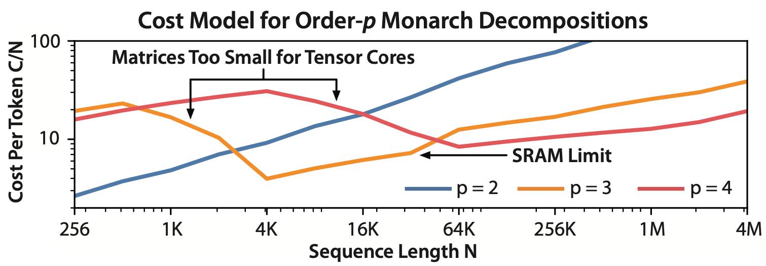
Cost of various different order- FFT convolutions for different sequence lengths.
- You can see that for short sequences (shorter than 4K), an order-2 decomposition is fine, since it allows us to break the FFT down into 16x16 matmuls – but quickly grows more expensive for longer sequences.
- Meanwhile, higher-order decompositions can’t fully use the tensor cores for short sequences – but better asymptotic scaling kicks in for longer sequences.
- You can also see the kink in the orange line that arises from the SRAM limit – the 4th-order Monarch allows us to break past the SRAM limit!
Speeding Up Convolutional Models with FlashFFTConv
So what does this change in algorithm buy you? Faster convolutions, and faster convolutional sequence models! We’ll present some brief highlights here, but check out our paper for more details!
Faster End-to-End Models
We benchmark end-to-end speedup with FlashFFTConv. This table shows throughput in sequences per second, between PyTorch and FlashFFTConv on a single H100. FlashFFTConv speeds up convolutional sequence models end-to-end – up to 4.4X for HyenaDNA!
| Model (size, seqlen) | PyTorch | FlashFFTConv | Speedup |
|---|---|---|---|
| M2-BERT-base (110M, 128) | 4480 | 8580 | 1.9x |
| Hyena-s-4K (155M, 4K) | 84.1 | 147 | 1.7x |
| HyenaDNA (6M, 1M) | 0.69 | 3.03 | 4.4x |
Check out the examples in our code base for examples of how to adapt these models for FlashFFTConv. FlashFFTConv has already been integrated into a number of research codebases, and we’ll be excited to announce a number of new models that were trained with FlashFFTConv, coming out soon!
Speedups over FlashAttention-v2
Thanks to these optimizations, convolutional language models are now starting to match the most optimized Transformers end-to-end, even for sequences as short as 2K.
Here, we compare the throughput in toks/ms, and FLOP utilization of Hyena running FlashFFTConv compared to FlashAttention-v2 for some 3B-equivalent models across sequence lengths:
| Model | 2K | 8K | 16K |
|---|---|---|---|
| GPT-2.7B, FA-v2 Throughput | 33.8 | 27.8 | 21.6 |
| Hyena-2.7B, FlashFFTConv Throughput | 35.2 | 35.2 | 32.3 |
| FA-v2 FLOP Util | 65.7 | 72.1 | 78.5 |
| FlashFFTConv Flop Util | 62.3 | 61.9 | 56.5 |
| Speedup | 1.1x | 1.3x | 1.5x |
FlashFFTConv achieves up to 62% MFU – and is faster than FlashAttention-v2 end-to-end due to a lower FLOP cost!
What's Next
You can try out FlashFFTConv now - we welcome feedback about where it’s useful, or where it could be further improved. We’re super excited about this intersection of new architectures and new systems algorithms to support them on modern hardware.
Check out our paper for a deeper dive into the algorithms – and some discussion about how this systems advance can also push the boundaries of ML algorithms, with sparse convolutions that are naturally enabled by FlashFFTConv (we just skip parts of the matrices).
And watch for more work releasing soon that uses FlashFFTConv!
If you’re excited by these directions, please reach out – we would love to chat!
Dan Fu: danfu@cs.stanford.edu; Hermann Kumbong: kumboh@stanford.edu